3.1. Bulk Processing of Multiple NNI Series with pyHRV
This tutorial aims to guide you through all the steps needed to bulk process multiple NNI series using a simple Python script. This can be helpful in one of the following examples (there exist of course many other cases for which this might be useful:
- You need to analyse datasets from multiple participants joining your experiment
- Over time, multiple new participants join your experiment and you need to compute their datasets
- The analysis process requires you to test different input settings, such as for example adjusting the selected frequency bands or filter orders, which requires you to recompute the HRV parameters with each change being made to the intput
- Any other reason that you might think of needing bulk processing…
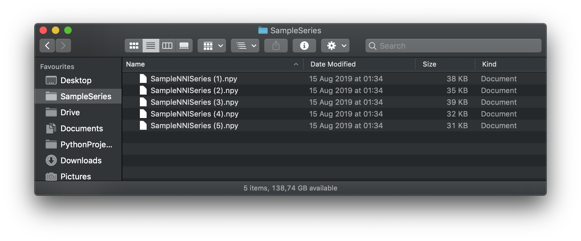
For instance, I have a couple of files with NNI series stored in the .npy numpy array format which I would like to process using the same input settings.
3.1.1. Step 1: Loading the Necessary Packages
We will require the following 3 packages in this script:
- glob to loop through all the files containing the NNI series in a folder
- numpy to load the NNI series
- pyHRV to compute the HRV results
import glob
import pyhrv
import numpy as np
3.1.2. Step 2: Defining the Input Parameters for the HRV Functions
pyHRV’s functions already come with default values for input parameters. However, the use of custom input values is often interesting in order to adjust the functions to the experimental conditions.
In this step, we will prepare a series of dictionaries containing the input parameters for the computation of Time Domain, Frequency Domain and Nonlinear parameters. These dictionaries will afterwards be used with the pyhrv.hrv() (see The HRV Function: hrv()).
First, we prepare the inputs for the Time Domain functions:
# Time Domain Settings
settings_time = {
    'threshold': 50,            # Computation of NNXX/pNNXX with 50 ms threshold -> NN50 & pNN50
    'plot': True,               # If True, plots NNI histogram
    'binsize': 7.8125           # Binsize of the NNI histogram
}
For the Frequency Domain parameters, we will prepare individual input dictionaries for each of the available functions, Welch’s Method: welch_psd(), Lomb-Scargle Periodogram: lomb_psd() and Autoregressive Method: ar_psd().
# Frequency Domain Settings
settings_welch = {
    'nfft': 2 ** 12,            # Number of points computed for the FFT result
    'detrend': True,            # If True, detrend NNI series by subtracting the mean NNI
    'window': 'hanning'         # Window function used for PSD estimation
}

settings_lomb = {
    'nfft': 2**8,               # Number of points computed for the Lomb PSD
    'ma_size': 5                # Moving average window size
}

settings_ar = {
    'nfft': 2**12,              # Number of points computed for the AR PSD
    'order': 32                 # AR order
}
At last, we will set the input parameters for the Nonlinear Parameters.
# Nonlinear Parameter Settings
settings_nonlinear = {
    'short': [4, 16],           # Interval limits of the short term fluctuations
    'long': [17, 64],           # Interval limits of the long term fluctuations
    'dim': 2,                   # Sample entropy embedding dimension
    'tolerance': None           # Tolerance distance for which the vectors to be considered equal (None sets default values)
}
Tip
Storing the settings in multiple dictionaries within a Python script might become unhandy if you would like to share your settings or simply keep those out of a Python script for more versatility.
In those cases, store the settings in a JSON file which can be easily read with Python’s native JSON Package.
3.1.3. Step 3: Looping Through All the Available Files
In this step, we will create a loop which to go through all the available files and load the NNI series from each file which we then use to compute the HRV parameters.
For this, we will first define the path where the files are stored. Afterwards, we will loop through all the files using the glob package.
# Path where the NNI series are stored
nni_data_path = './SampleSeries/'

# Go through all files in the folder (here: files that end with .npy only)
for nni_file in glob.glob(nni_data_path + '*.npy'):

    # Load the NNI series of the current file
    nni = np.load(nni_file)
3.1.4. Step 4: Computing the HRV parameters
At last, we will pass the previously defined input parameters to the pyhrv.hrv() function and compute the HRV parameters.
# Path where the NNI series are stored
nni_data_path = './SampleSeries/'

# Go through all files in the folder (here: that end with .npy)
for nni_file in glob.glob(nni_data_path + '*.npy'):

   # Load the NNI series of the current file
   nni = np.load(nni_file)

   # Compute the pyHRV parameters
   results = pyhrv.hrv(nni=nni,
                       kwargs_time=settings_time,
                       kwargs_welch=settings_welch,
                       kwargs_ar=settings_ar,
                       kwargs_lomb=settings_lomb,
                       kwargs_nonlinear=settings_nonlinear)
That’s it! Now adjust the script to your needs so that the computed results can be used as you need those for your project.
3.1.5. Tl;dr - The Entire Script
The code sections we have generated over the course of this tutorial are summarized in the following Python script:
# Import necessary packages
import glob
import pyhrv
import numpy as np

# Define HRV input parameters
# Time Domain Settings
settings_time = {
    'threshold': 50,            # Computation of NNXX/pNNXX with 50 ms threshold -> NN50 & pNN50
    'plot': True,               # If True, plots NNI histogram
    'binsize': 7.8125           # Binsize of the NNI histogram
}

# Frequency Domain Settings
settings_welch = {
    'nfft': 2 ** 12,            # Number of points computed for the FFT result
    'detrend': True,            # If True, detrend NNI series by subtracting the mean NNI
    'window': 'hanning'         # Window function used for PSD estimation
}

settings_lomb = {
    'nfft': 2**8,               # Number of points computed for the Lomb PSD
    'ma_size': 5                # Moving average window size
}

settings_ar = {
    'nfft': 2**12,              # Number of points computed for the AR PSD
    'order': 32                 # AR order
}

# Nonlinear Parameter Settings
settings_nonlinear = {
    'short': [4, 16],           # Interval limits of the short term fluctuations
    'long': [17, 64],           # Interval limits of the long term fluctuations
    'dim': 2,                   # Sample entropy embedding dimension
    'tolerance': None           # Tolerance distance for which the vectors to be considered equal (None sets default values)
}

# Path where the NNI series are stored
nni_data_path = './SampleSeries/'

# Go through all files in the folder (here: that end with .npy)
for nni_file in glob.glob(nni_data_path + '*.npy'):

   # Load the NNI series of the current file
   nni = np.load(nni_file)

   # Compute the pyHRV parameters
   results = pyhrv.hrv(nni=nni,
                       kwargs_time=settings_time,
                       kwargs_welch=settings_welch,
                       kwargs_ar=settings_ar,
                       kwargs_lomb=settings_lomb,
                       kwargs_nonlinear=settings_nonlinear)
Note
Any feedback or ideas how to improve this tutorial? Feel free to share your ideas or questions with me via e-mail: pgomes92@gmail.com