2.4. Frequency Domain Module ¶

The Frequency Domain Module contains all functions to compute the frequency domain parameters derived from the PSD estimation using the Welch’s method, the Lomb-Scargle Periodogram and the Autoregressive method.

Module Contents

Frequency Domain Module

See also

2.4.1. Welch’s Method: welch_psd()¶

pyhrv.frequency_domain.welch_psd(nn=None, rpeaks=None, fbands=None, nfft=2**12, detrend=True, window='hamming', show=True, show_param=True, legend=True)¶

Function Description

Computes a Power Spectral Density (PSD) estimation from the NNI series using the Welch’s method and computes all frequency domain parameters from this PSD according to the specified frequency bands.

If no frequency bands are specified, the default frequency band limits for the Very Low Frequency (VLF), Low Frequency (LF), and High Frequency (HF) bands as recommended by the HRV Guidelines are applied:

VLF: [0.00Hz - 0.04Hz]

LF: [0.04Hz - 0.15Hz]

HF: [0.15Hz - 0.40Hz]

Use the fbands parameter to specify custom frequency bands and the possibility to add the Ultra Low Frequency (ULF) band (see Application Notes & Examples & Tutorials below for more information).

The following parameters are computed from the PSD and the specified frequency bands:

Peak frequencies [Hz]

Absolute powers [ms^2]

Relative powers [ms^2]

Logarithmic powers [log]

Normalized powers (LF & HF only)[-]

Total power of all frequency bands [ms^2]

An example of a PSD plot generated by this function can be seen here:

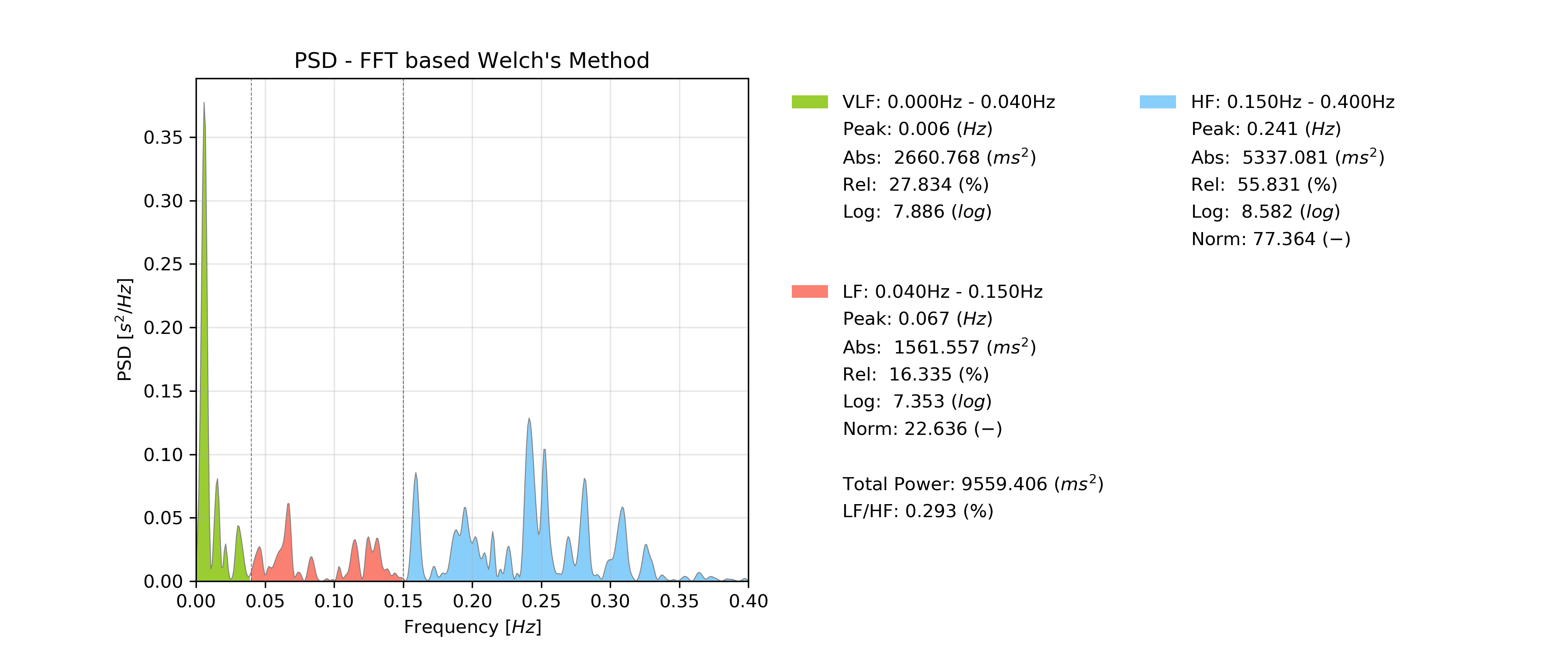
Sample Welch PSD.

Input Parameters

nn (array): NN intervals in [ms] or [s]
rpeaks (array): R-peak times in [ms] or [s]
fbands (dict, optional): Dictionary with frequency band specifications (default: None)
nfft (int, optional): Number of points computed for the FFT result (default: 2**12)
detrend (bool, optional): If True, detrend NNI series by subtracting the mean NNI (default: True)
window (scipy.window function, optional): Window function used for PSD estimation (default: ‘hamming’)
show (bool, optional): If True, show PSD plot figure (default: True)
show_param (bool, optional): If true, list all computed PSD parameters next to the plot (default: True)
legend (bool, optional): If true, add a legend with frequency bands to the plot (default: True)

Note

If fbands is none, the default values for the frequency bands will be set.

VLF: [0.00Hz - 0.04Hz]

LF: [0.04Hz - 0.15Hz]

HF: [0.15Hz - 0.40Hz]

See Application Notes & Examples & Tutorials below for more information on how to define custom frequency bands.

Important

The specified nfft refers to the overall number of samples computed for the entire PSD estimation regardless of frequency bands, i.e. the number of samples within the lowest and the highest frequency band limit is not necessarily equal to the specified nfft.

Returns (ReturnTuple Object)

The results of this function are returned in a biosppy.utils.ReturnTuple object. Use the keys below (on the left) to index the results:

fft_peak (tuple): Peak frequencies of all frequency bands [Hz]

fft_abs (tuple): Absolute powers of all frequency bands [ms^2]

fft_rel (tuple): Relative powers of all frequency bands [%]

fft_log (tuple): Logarithmic powers of all frequency bands [log]

fft_norm (tuple): Normalized powers of the LF and HF frequency bands [-]

fft_ratio (float): LF/HF ratio [-]

fft_total (float): Total power over all frequency bands [ms^2]

fft_interpolation (str): Interpolation method used for NNI interpolation (hard-coded to ‘cubic’)

fft_resampling_frequency (int): Resampling frequency used for NNI interpolation [Hz] (hard-coded to 4Hz as recommended by the HRV Guidelines)

fft_window (str): Spectral window used for PSD estimation of the Welch’s method

fft_plot (matplotlib figure object): PSD plot figure object

See also

The biosppy.utils.ReturnTuple Object

Computation Method

This functions computes the PSD estimation using the scipy.signals.lomb() (docs, source) function.

The flowchart below visualizes the structure of this function. The NNI series are interpolated at a new sampling frequency of 4Hz before the PSD computation as per the HRV guidelines.

See also

Section ref-freqparams for detailed information about the computation of the individual parameters.

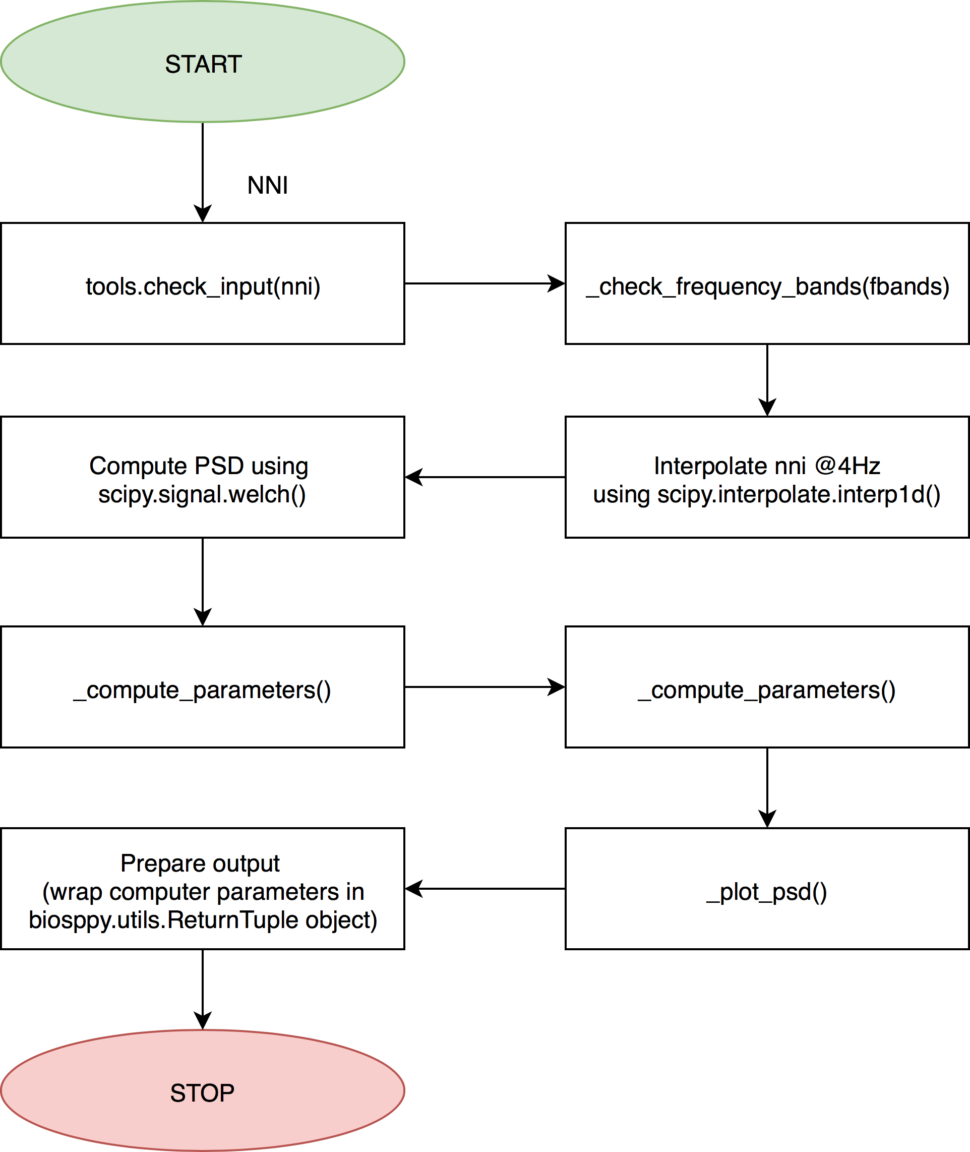
Flowchart of the welch_psd() function.

Application Notes

It is not necessary to provide input data for nni and rpeaks. The parameter(s) of this function will be computed with any of the input data provided (nni or rpeaks). nni will be prioritized in case both are provided.

nni or rpeaks data provided in seconds [s] will automatically be converted to nni data in milliseconds [ms].

See also

Section NN Format: nn_format() for more information.

Incorrect frequency band specifications will be automatically corrected, if possible. For instance the following frequency bands contain overlapping frequency band limits which would cause issues when computing the frequency parameters:

fbands = {'vlf': (0.0, 0.25), 'lf': (0.2, 0.3), 'hf': (0.3, 0.4)}

Here, the upper band of the VLF band is greater than the lower band of the LF band. In this case, the overlapping frequency band limits will be switched:

fbands = {'vlf': (0.0, 0.2), 'lf': (0.25, 0.3), 'hf': (0.3, 0.4)}

Warning

Corrections of frequency bands trigger warnings which are displayed in the Python console. It is recommended to watch out for these warnings and to correct the frequency bands given that the corrected bands might not be optimal.

This issue is shown in the following PSD plot where the corrected frequency bands above were used and there is no frequency band covering the range between 0.2Hz and 0.25Hz:

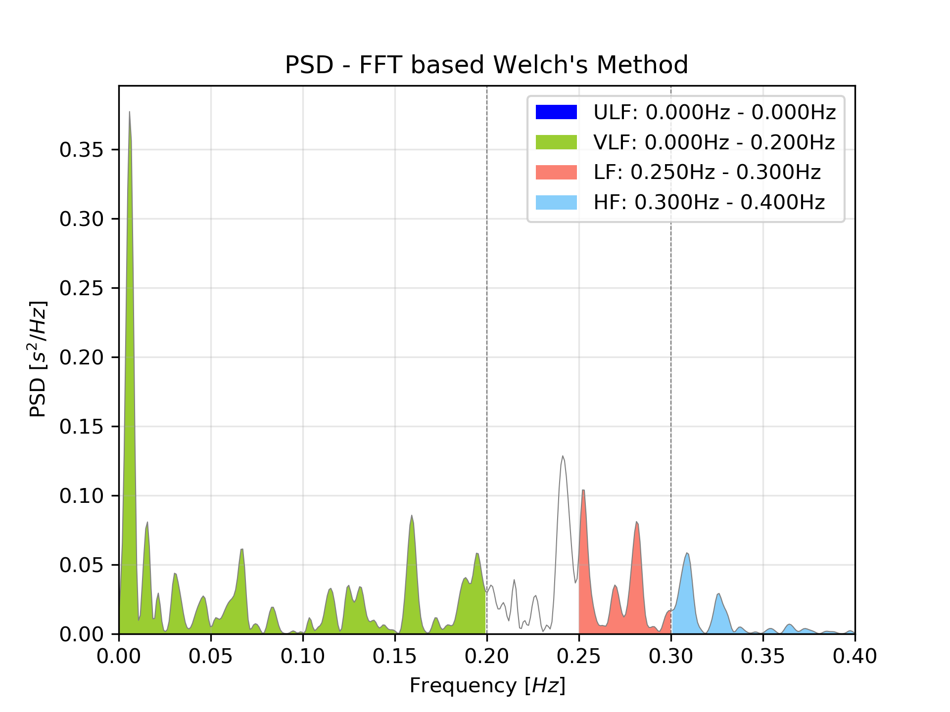
Welch PSD with corrected frequency bands and frequency band gaps.

The resampling frequency and the interpolation methods used for this method are hardcoded to 4Hz and the cubic spline interpolation of the scipy.interpolate.interp1d() (docs, source) function.

Important

This function generates matplotlib plot figures which, depending on the backend you are using, can interrupt your code from being executed whenever plot figures are shown. Switching the backend and turning on the matplotlib interactive mode can solve this behavior.

In case it does not - or if switching the backend is not possible - close all the plot figures to proceed with the execution of the rest your code after the plt.show().

See also

Examples & Tutorials

The following example code demonstrates how to use this function and how access the results stored in the biosppy.utils.ReturnTuple object.

You can use NNI series (nni) to compute the PSD:

# Import packages
import pyhrv
import pyhrv.frequency_domain as fd

# Load NNI sample series
pyhrv.utils.load_sample_nni()

# Compute the PSD and frequency domain parameters using the NNI series
result = fd.welch_psd(nni)

# Access peak frequencies using the key 'fft_peak'
print(result['fft_peak'])

Alternatively, you can use R-peak series (rpeaks):

# Import packages
import biosppy
import pyhrv.frequency_domain as fd

# Load sample ECG signal
signal = np.loadtxt('./files/SampleECG.txt')[:, -1]

# Get R-peaks series using biosppy
t, filtered_signal, rpeaks = biosppy.signals.ecg.ecg(signal)[:3]

# Compute the PSD and frequency domain parameters using the R-peak series
result = fd.welch_psd(rpeaks=t[rpeaks])

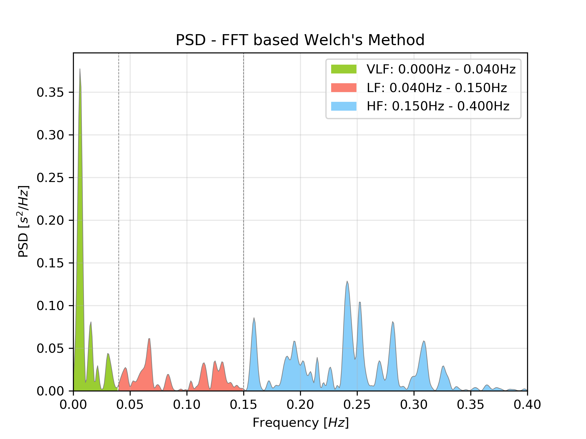
The plot of these examples should look like the following plot:

Welch PSD with default frequency bands.

If you want to specify custom frequency bands, define the limits in a Python dictionary as shown in the following example:

# Define custom frequency bands and add the ULF band
fbands = {'ulf': (0.0, 0.1), 'vlf': (0.1, 0.2), 'lf': (0.2, 0.3), 'hf': (0.3, 0.4)}

# Compute the PSD with custom frequency bands
result = fd.welch_psd(nni, fbands=fbands)

The plot of this example should look like the following plot:

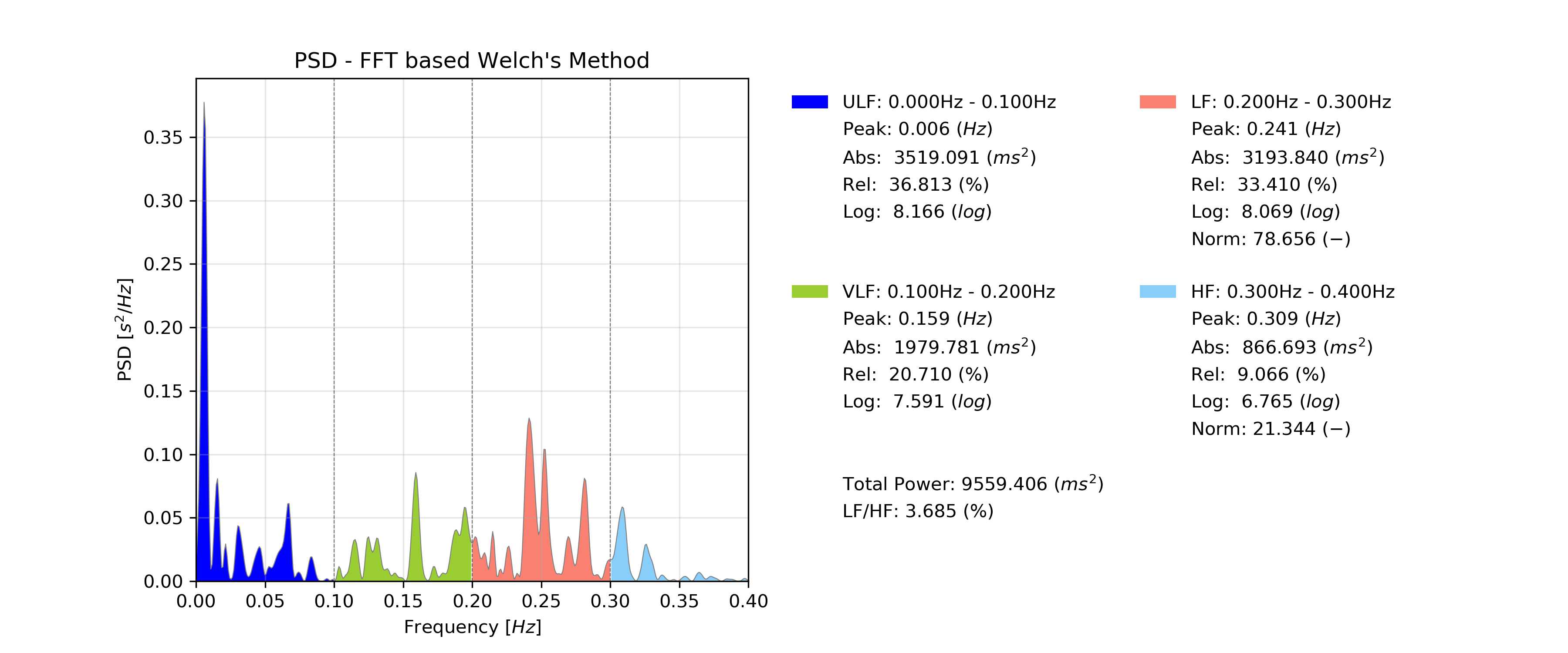
Welch PSD with custom frequency bands.

By default, the figure will contain the PSD plot on the left and the computed parameter results on the right side of the figure. Set the show_param to False if only the PSD is needed in the figure.

# Compute the PSD without the parameters being shown on the right side of the figure
result = fd.welch_psd(nni, show_param=False)

The plot for this example should look like the following plot:

PSD plot without parameters.

2.4.2. Lomb-Scargle Periodogram: lomb_psd()¶

pyhrv.frequency_domain.lomb_psd(nn=None, rpeaks=None, fbands=None, nfft=2**8, ma_size=None, show=True, show_param=True, legend=True)¶

Function Description

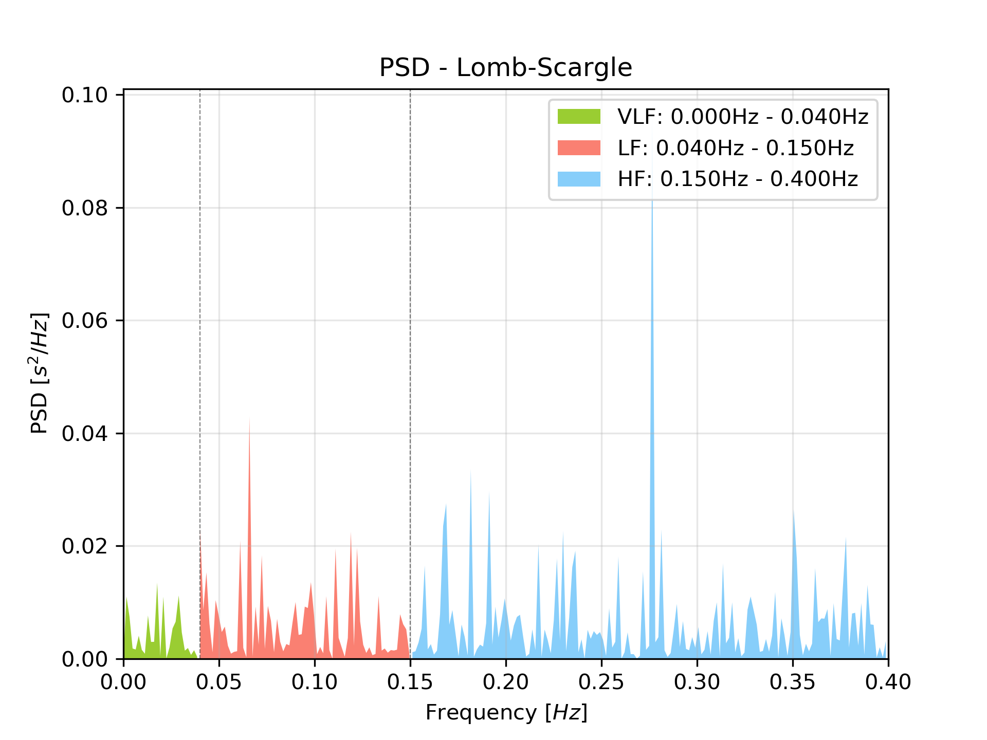
Computes a Power Spectral Density (PSD) estimation from the NNI series using the Lomb-Scargle Periodogram and computes all frequency domain parameters from this PSD according to the specified frequency bands.

If no frequency bands are specified, the default frequency band limits for the Very Low Frequency (VLF), Low Frequency (LF), and High Frequency (HF) bands as recommended by the HRV Guidelines are applied:

VLF: [0.00Hz - 0.04Hz]

LF: [0.04Hz - 0.15Hz]

HF: [0.15Hz - 0.40Hz]

Use the fbands parameter to specify custom frequency bands and the possibility to add the Ultra Low Frequency (ULF) band (see Application Notes & Examples & Tutorials below for more information).

The following parameters are determined from the PSD and the specified frequency bands:

Peak frequencies [Hz]

Absolute powers [ms^2]

Relative powers [ms^2]

Logarithmic powers [log]

Normalized powers (LF & HF only)[-]

Total power of all frequency bands [ms^2]

An example of a PSD plot generated by this function can be seen here:

Sample Lomb PSD.

Input Parameters

nn (array): NN intervals in [ms] or [s].
rpeaks (array): R-peak times in [ms] or [s].
fbands (dict, optional): Dictionary with frequency band specifications (default: None)
nfft (int, optional): Number of points computed for the Lomb-Scargle result (default: 2**8)
ma_order (int, optional): Order of the moving average filter (default: None; no filter applied)
show (bool, optional): If True, show PSD plot figure (default: True)
show_param (bool, optional): If true, list all computed PSD parameters next to the plot (default: True)
legend (bool, optional): If true, add a legend with frequency bands to the plot (default: True)

Note

If fbands is none, the default values for the frequency bands will be set:

VLF: [0.00Hz - 0.04Hz]

LF: [0.04Hz - 0.15Hz]

HF: [0.15Hz - 0.40Hz]

See Application Notes & Examples & Tutorials below to learn how to specify custom frequency bands.

Important

The specified nfft refers to the overall number of samples computed for the entire PSD estimation regardless of frequency bands, i.e. the number of samples within the lowest and the highest frequency band limit is not necessarily equal to the specified nfft.

Returns (ReturnTuple Object)

The results of this function are returned in a biosppy.utils.ReturnTuple object. Use the following keys below (on the left) to index the results:

lomb_peak (tuple): Peak frequencies of all frequency bands [Hz]

lomb_abs (tuple): Absolute powers of all frequency bands [ms^2]

lomb_rel (tuple): Relative powers of all frequency bands [%]

lomb_log (tuple): Logarithmic powers of all frequency bands [log]

lomb_norm (tuple): Normalized powers of the LF and HF frequency bands [-]

lomb_ratio (float): LF/HF ratio [-]

lomb_total (float): Total power over all frequency bands [ms^2]

lomb_ma (int): Moving average filter order [-]

lomb_plot (matplotlib figure object): PSD plot figure object

See also

The biosppy.utils.ReturnTuple Object

Computation Method

This functions computes the PSD estimation using the scipy.signals.lombscargle() (docs , source) function.

See also

Section ref-freqparams for detailed information about the computation of the individual parameters.

Application Notes

It is not necessary to provide input data for nni and rpeaks. The parameter(s) of this function will be computed with any of the input data provided (nni or rpeaks). nni will be prioritized in case both are provided.

nni or rpeaks data provided in seconds [s] will automatically be converted to nni data in milliseconds [ms].

See also

Section NN Format: nn_format() for more information.

Incorrect frequency band specifications will be automatically corrected, if possible. For instance the following frequency bands contain overlapping frequency band limits which would cause issues when computing the frequency parameters:

fbands = {'vlf': (0.0, 0.25), 'lf': (0.2, 0.3), 'hf': (0.3, 0.4)}

Here, the upper band of the VLF band is greater than the lower band of the LF band. In this case, the overlapping frequency band limits will be switched:

fbands = {'vlf': (0.0, 0.2), 'lf': (0.25, 0.3), 'hf': (0.3, 0.4)}

Warning

Corrections of frequency bands trigger warnings which are displayed in the Python console. It is recommended to watch out for these warnings and to correct the frequency bands given that the corrected bands might not be optimal.

This issue is shown in the following PSD plot where the corrected frequency bands above were used and there is no frequency band covering the range between 0.2Hz and 0.25Hz:

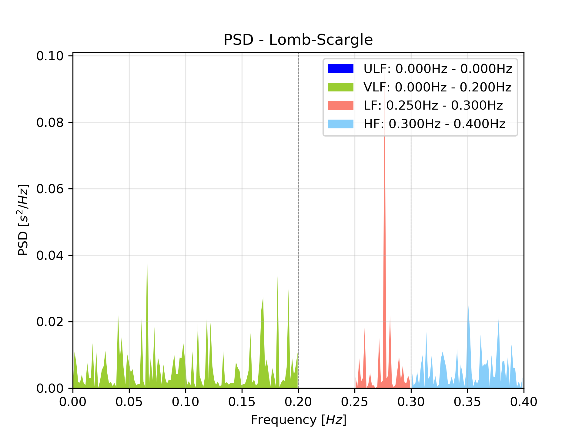
Lomb PSD with corrected frequency bands and frequency band gaps.

Important

This function generates matplotlib plot figures which, depending on the backend you are using, can interrupt your code from being executed whenever plot figures are shown. Switching the backend and turning on the matplotlib interactive mode can solve this behavior.

In case it does not - or if switching the backend is not possible - close all the plot figures to proceed with the execution of the rest your code after the plt.show() function.

See also

Examples & Tutorials

The following example code demonstrates how to use this function and how access the results stored in the biosppy.utils.ReturnTuple object.

You can use NNI series (nni) to compute the PSD:

# Import packages
import pyhrv
import pyhrv.frequency_domain as fd

# Load NNI sample series
pyhrv.utils.load_sample_nni()

# Compute the PSD and frequency domain parameters using the NNI series
result = fd.lomb_psd(nni)

# Access peak frequencies using the key 'lomb_peak'
print(result['lomb_peak'])

Alternatively, you can use R-peak series (rpeaks):

# Import packages
import biosppy
import pyhrv.frequency_domain as fd

# Load sample ECG signal
signal = np.loadtxt('./files/SampleECG.txt')[:, -1]

# Get R-peaks series using biosppy
t, filtered_signal, rpeaks = biosppy.signals.ecg.ecg(signal)[:3]

# Compute the PSD and frequency domain parameters using the R-peak series
result = fd.lomb_psd(rpeaks=t[rpeaks])

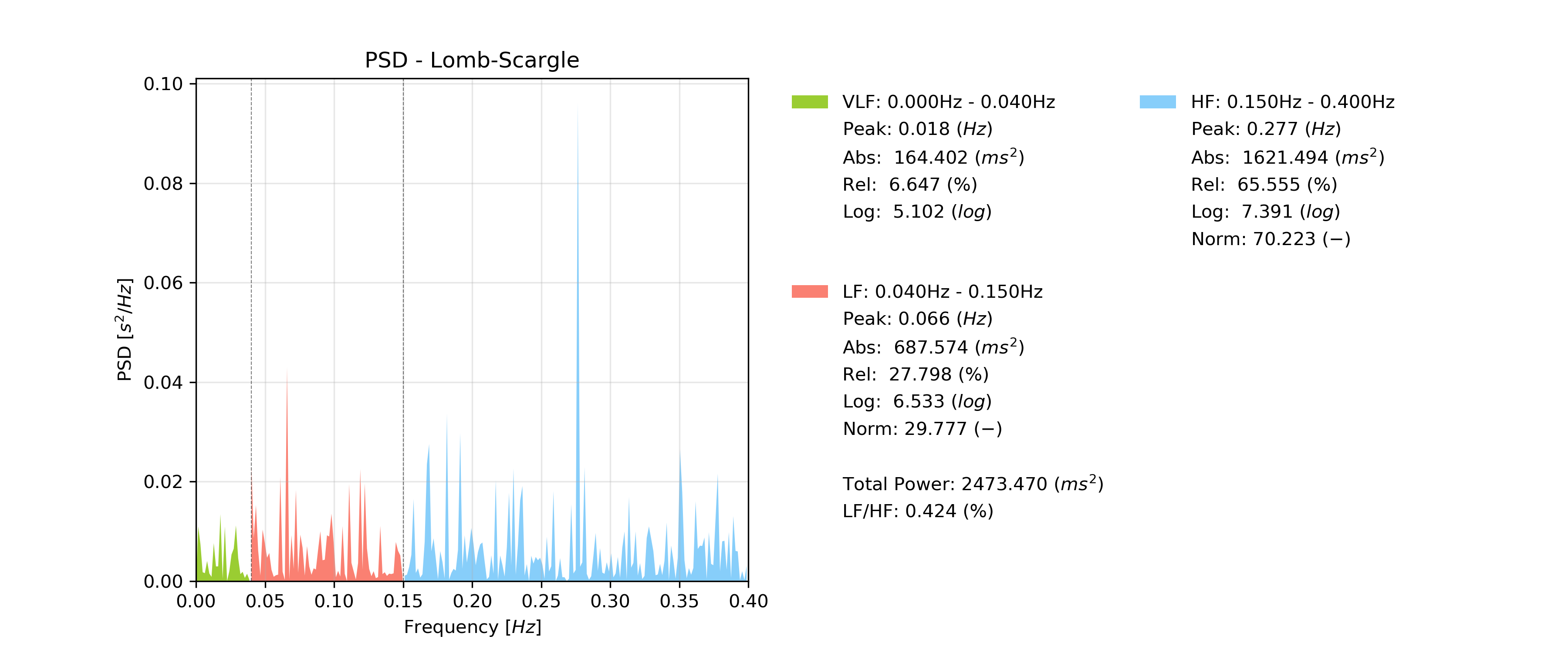
The plot of these examples should look like the following plot:

Lomb PSD with default frequency bands.

If you want to specify custom frequency bands, define the limits in a Python dictionary as shown in the following example:

# Define custom frequency bands and add the ULF band
fbands = {'ulf': (0.0, 0.1), 'vlf': (0.1, 0.2), 'lf': (0.2, 0.3), 'hf': (0.3, 0.4)}

# Compute the PSD with custom frequency bands
result = fd.lomb_psd(nni, fbands=fbands)

The plot of this example should look like the following plot:

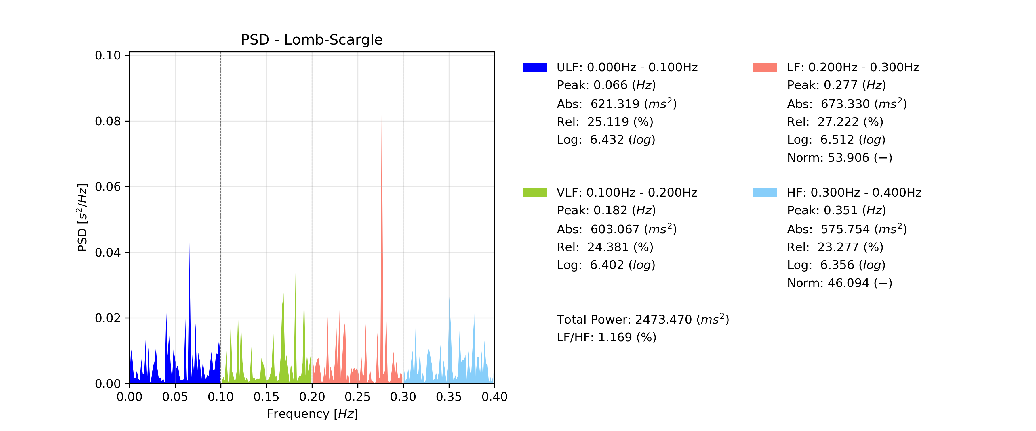
Lomb PSD with custom frequency bands.

By default, the figure will contain the PSD plot on the left and the computed parameter results on the right side of the figure. Set the show_param to False if only the PSD is needed in the figure.

# Compute the PSD without the parameters being shown on the right side of the figure
result = fd.lomb_psd(nni, show_param=False)

The plot for this example should look like the following plot:

Lomb PSD without parameters.

2.4.3. Autoregressive Method: ar_psd()¶

pyhrv.frequency_domain.ar_psd(nn=None, rpeaks=None, fbands=None, nfft=2**12, order=16, show=True, show_param=True, legend=True)¶

Function Description

Computes a Power Spectral Density (PSD) estimation from the NNI series using the Autoregressive method and computes all frequency domain parameters from this PSD according to the specified frequency bands.

If no frequency bands are specified, the default frequency band limits for the Very Low Frequency (VLF), Low Frequency (LF), and High Frequency (HF) bands as recommended by the HRV Guidelines are applied:

VLF: [0.00Hz - 0.04Hz]

LF: [0.04Hz - 0.15Hz]

HF: [0.15Hz - 0.40Hz]

Use the fbands parameter to specify custom frequency bands and the possibility to add the Ultra Low Frequency (ULF) band (see Application Notes & Examples & Tutorials below for more information).

The following parameters are computed from the PSD and the specified frequency bands:

Peak frequencies [Hz]

Absolute powers [ms^2]

Relative powers [ms^2]

Logarithmic powers [log]

Normalized powers (LF & HF only)[-]

Total power of all frequency bands [ms^2]

An example of a PSD plot generated by this function can be seen here:

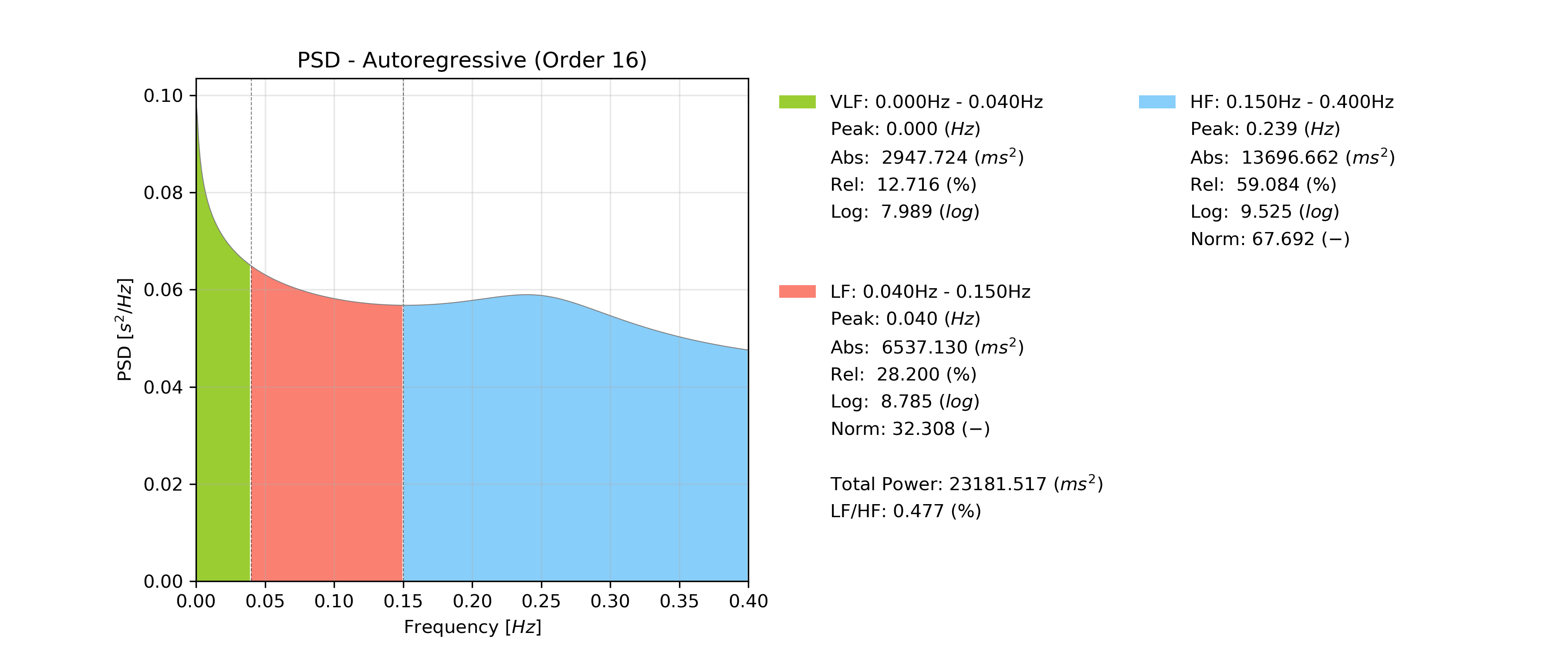
Sample Autoregressive PSD.

Input Parameters

nn (array): NN intervals in [ms] or [s].
rpeaks (array): R-peak times in [ms] or [s].
fbands (dict, optional): Dictionary with frequency band specifications (default: None)
nfft (int, optional): Number of points computed for the FFT result (default: 2**12)
order (int, optional): Autoregressive model order (default: 16)
show (bool, optional): If True, show PSD plot figure (default: True)
show_param (bool, optional): If true, list all computed PSD parameters next to the plot (default: True)
legend (bool, optional): If true, add a legend with frequency bands to the plot (default: True)

Note

If fbands is none, the default values for the frequency bands will be set.

VLF: [0.00Hz - 0.04Hz]

LF: [0.04Hz - 0.15Hz]

HF: [0.15Hz - 0.40Hz]

See Application Notes & Examples & Tutorials below for more information on how to define custom frequency bands.

Important

The specified nfft refers to the overall number of samples computed for the entire PSD estimation regardless of frequency bands, i.e. the number of samples within the lowest and the highest frequency band limit is not necessarily equal to the specified nfft.

Returns (ReturnTuple Object)

The results of this function are returned in a biosppy.utils.ReturnTuple object. Use the following keys below (on the left) to index the results:

ar_peak (tuple): Peak frequencies of all frequency bands [Hz]

ar_abs (tuple): Absolute powers of all frequency bands [ms^2]

ar_rel (tuple): Relative powers of all frequency bands [%]

ar_log (tuple): Logarithmic powers of all frequency bands [log]

ar_norm (tuple): Normalized powers of the LF and HF frequency bands [-]

ar_ratio (float): LF/HF ratio [-]

ar_total (float): Total power over all frequency bands [ms^2]

ar_interpolation (str): Interpolation method used for NNI interpolation (hard-coded to ‘cubic’)

ar_resampling_frequency (int): Resampling frequency used for NNI interpolation [Hz] (hard-coded to 4Hz as recommended by the HRV Guidelines)

ar_window (str): Spectral window used for PSD estimation of the Welch’s method

ar_order (int): Autoregressive model order

ar_plot (matplotlib figure object): PSD plot figure object

See also

The biosppy.utils.ReturnTuple Object

Computation Method

This functions computes the PSD estimation using the spectrum.pyule() (docs, source) function.

The flowchart below visualizes the structure of the ar_psd() function. The NNI series are interpolated at a new sampling frequency of 4Hz before the PSD computation is conducted as the unevenly sampled NNI series would distort the PSD.

See also

Section ref-freqparams for detailed information about the computation of the individual parameters.

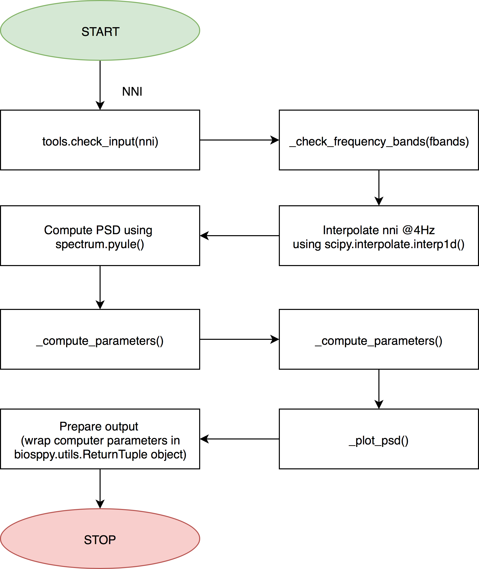
Flowchart of the ar_psd() function.

Application Notes

It is not necessary to provide input data for nni and rpeaks. The parameter(s) of this function will be computed with any of the input data provided (nni or rpeaks). nni will be prioritized in case both are provided.

nni or rpeaks data provided in seconds [s] will automatically be converted to nni data in milliseconds [ms].

See also

Section NN Format: nn_format() for more information.

Incorrect frequency band specifications will be automatically corrected, if possible. For instance the following frequency bands contain overlapping frequency band limits which would cause issues when computing the frequency parameters:

fbands = {'vlf': (0.0, 0.25), 'lf': (0.2, 0.3), 'hf': (0.3, 0.4)}

Here, the upper band of the VLF band is greater than the lower band of the LF band. In this case, the overlapping frequency band limits will be switched:

fbands = {'vlf': (0.0, 0.2), 'lf': (0.25, 0.3), 'hf': (0.3, 0.4)}

Warning

Corrections of frequency bands trigger warnings which are displayed in the Python console. It is recommended to watch out for these warnings and to correct the frequency bands given that the corrected bands might not be optimal.

This issue is shown in the following PSD plot where the corrected frequency bands above were used and there is no frequency band covering the range between 0.2Hz and 0.25Hz:

Autoregressive PSD with corrected frequency bands and frequency band gaps.

The resampling frequency and the interpolation methods used for this method are hardcoded to 4Hz and the cubic spline interpolation of the scipy.interpolate.interp1d() (docs, source) function.

Important

This function generates matplotlib plot figures which, depending on the backend you are using, can interrupt your code from being executed whenever plot figures are shown. Switching the backend and turning on the matplotlib interactive mode can solve this behavior.

In case it does not - or if switching the backend is not possible - close all the plot figures to proceed with the execution of the rest your code after the plt.show() function.

See also

Examples & Tutorials

The following example code demonstrates how to use this function and how access the results stored in the biosppy.utils.ReturnTuple object.

You can use NNI series (nni) to compute the PSD:

# Import packages
import pyhrv
import pyhrv.frequency_domain as fd

# Load NNI sample series
pyhrv.utils.load_sample_nni()

# Compute the PSD and frequency domain parameters using the NNI series
result = fd.ar_psd(nni)

# Access peak frequencies using the key 'ar_peak'
print(result['ar_peak'])

Alternatively, you can use R-peak series (rpeaks):

# Import packages
import biosppy
import pyhrv.frequency_domain as fd

# Load sample ECG signal
signal = np.loadtxt('./files/SampleECG.txt')[:, -1]

# Get R-peaks series using biosppy
t, filtered_signal, rpeaks = biosppy.signals.ecg.ecg(signal)[:3]

# Compute the PSD and frequency domain parameters using the R-peak series
result = fd.ar_psd(rpeaks=t[rpeaks])

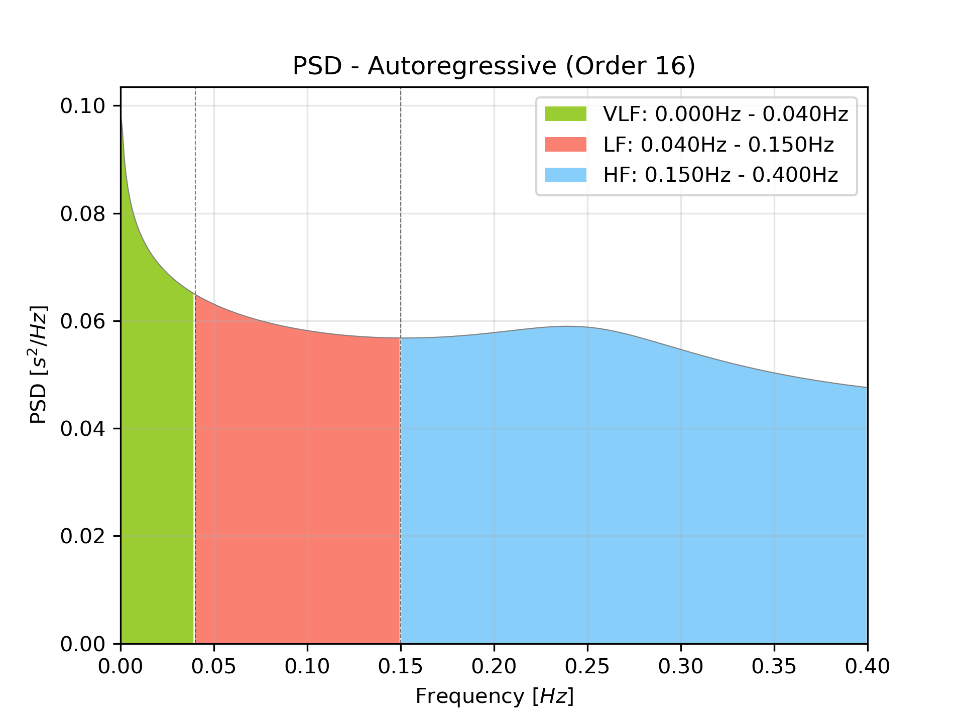
Autoregressive PSD with default frequency bands.

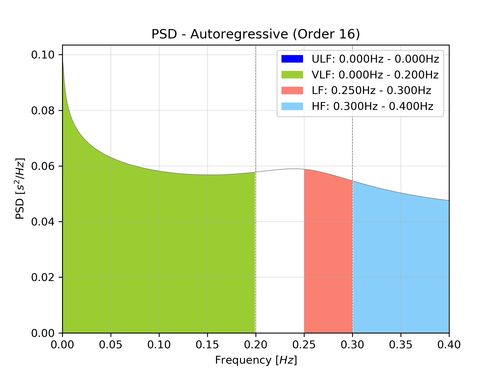
If you want to specify custom frequency bands, define the limits in a Python dictionary as shown in the following example:

# Define custom frequency bands and add the ULF band
fbands = {'ulf': (0.0, 0.1), 'vlf': (0.1, 0.2), 'lf': (0.2, 0.3), 'hf': (0.3, 0.4)}

# Compute the PSD with custom frequency bands
result = fd.ar_psd(nni, fbands=fbands)

# Access peak frequencies using the key 'ar_peak'
print(result['ar_peak'])

The plot of this example should look like the following plot:

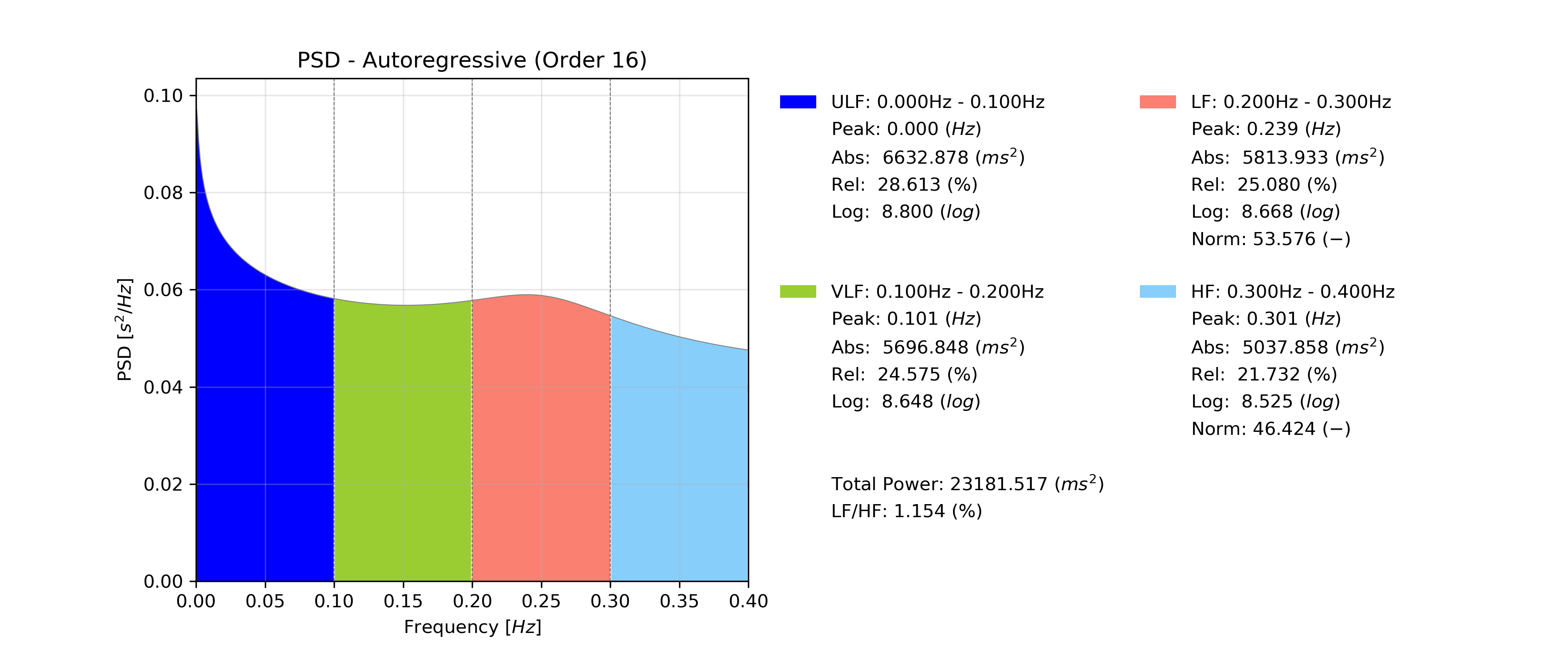
Autoregressive PSD with custom frequency bands.

By default, the figure will contain the PSD plot on the left and the computed parameter results on the left side of the figure. Set the show_param to False if only the PSD is needed in the figure.

# Compute the PSD without the parameters being shown on the right side of the figure
result = fd.ar_psd(nni, show_param=False)

# Access peak frequencies using the key 'ar_peak'
print(result['ar_peak'])

The plot for this example should look like the following plot:

PSD plot without parameters.

2.4.4. 2D PSD Comparison Plot: psd_comparison()¶

pyhrv.frequency_domain.psd_comparison(nni=None, rpeaks=None, segments=None, method='welch', fbands=None, duration=300, show=True, kwargs=None)¶

Function Description

Computes a series of PSDs from NNI segments extracted from a NNI/R-Peak input series or a series of input NNI segments and plots the result in a single plot. The PSDs are computed using the welch_psd(), lomb_psd(), or ar_psd() functions presented above.

This function aims to facilitate the visualization, comparison, and analyis of PSD evolution over time or NNI segments.

An example of a PSD comparison plot generated by this function can be seen here:

Sample PSD comparison plot.

See also

Welch’s Method: welch_psd()
Lomb-Scargle Periodogram: lomb_psd()
Autoregressive Method: ar_psd()

If no frequency bands are specified, the default frequency band limits for the Very Low Frequency (VLF), Low Frequency (LF), and High Frequency (HF) bands as recommended by the HRV Guidelines are applied:

VLF: [0.00Hz - 0.04Hz]

LF: [0.04Hz - 0.15Hz]

HF: [0.15Hz - 0.40Hz]

Use the fbands parameter to specify custom frequency bands and the possibility to add the Ultra Low Frequency (ULF) band (see Application Notes & Examples & Tutorials below for more information).

The following parameters are computed from the PSDs and the specified frequency bands for each segment:

Peak frequencies [Hz]

Absolute powers [ms^2]

Relative powers [ms^2]

Logarithmic powers [log]

Normalized powers (LF & HF only)[-]

Total power of all frequency bands [ms^2]

Input Parameters

nni (array): NN intervals in [ms] or [s]
rpeaks (array): R-peak times in [ms] or [s]
segments (array of arrays): Array containing pre-selected segments for the PSD computation in [ms] or [s]
method (str): PSD estimation method (‘welch’, ‘ar’ or ‘lomb’)
fbands (dict, optional): Dictionary with frequency band specifications (default: None)
duration (int): Maximum duration duration per segment in [s] (default: 300s)
show (bool, optional): If True, show PSD plot figure (default: True)
kwargs_method (dict): Dictionary of kwargs for the PSD computation functions ‘welch_psd()’, ‘ar_psd()’ or ‘lomb_psd()’

Note

If fbands is none, the default values for the frequency bands will be set.

VLF: [0.00Hz - 0.04Hz]

LF: [0.04Hz - 0.15Hz]

HF: [0.15Hz - 0.40Hz]

See Application Notes & Examples & Tutorials below for more information on how to define custom frequency bands.

Returns (ReturnTuple Object)

The results of this function are returned in a nested biosppy.utils.ReturnTuple object with the following structure:

psd_comparison_plot (matplotlib figure): Plot figure of the 2D comparison plot

segN (dict): Plot data and PSD parameters of the segment N

The segN contains the Frequency Domain parameter results computed from the segment N. The segments have number keys (e.g. first segment = seg0, second segment = seg0, …, last segment = segN).

Example of a 2-segment output:

'seg0': {
        # Frequency Domain parameters of the first segment (e.g., 'fft_peak', 'fft_abs', 'fft_log', etc.)
}
'seg1': {
        # Frequency Domain parameters of the second segment (e.g., 'fft_peak', 'fft_abs', 'fft_log', etc.)
}
'psd_comparison_plot': # matplotlib figure of the comparison plot

See also

The biosppy.utils.ReturnTuple Object

Important

If the the selected duration exceeds the overall duration of the input NNI series, the standard PSD plot and frequency domain results of the selected PDS method will be returned.

Keep an eye for warnings indicating if this is the case, as the output of this function will then provide the same output as the welch_psd(), lomb_psd() or ar_psd().

The kwargs_method input parameter will not have any effect in such cases.

Application Notes

It is not necessary to provide input data for nni and rpeaks. The parameter(s) of this function will be computed with any of the input data provided (nni or rpeaks). nni will be prioritized in case both are provided.

nni or rpeaks data provided in seconds [s] will automatically be converted to nni data in milliseconds [ms].

Segments will be chosen over ‘nni’ or ‘rpeaks’.

See also

Section NN Format: nn_format() for more information.

Incorrect frequency band specifications will be automatically corrected, if possible. For instance the following frequency bands contain overlapping frequency band limits which would cause issues when computing the frequency parameters:

fbands = {'vlf': (0.0, 0.25), 'lf': (0.2, 0.3), 'hf': (0.3, 0.4)}

Here, the upper band of the VLF band is greater than the lower band of the LF band. In this case, the overlapping frequency band limits will be switched:

fbands = {'vlf': (0.0, 0.2), 'lf': (0.25, 0.3), 'hf': (0.3, 0.4)}

Warning

Corrections of frequency bands trigger warnings which are displayed in the Python console. It is recommended to watch out for these warnings and to correct the frequency bands given that the corrected bands might not be optimal.

Important

This function generates matplotlib plot figures which, depending on the backend you are using, can interrupt your code from being executed whenever plot figures are shown. Switching the backend and turning on the matplotlib interactive mode can solve this behavior.

In case it does not - or if switching the backend is not possible - close all the plot figures to proceed with the execution of the rest your code after the plt.show().

See also

Examples & Tutorials

The following example code demonstrates how to use this function and how access the results stored in the biosppy.utils.ReturnTuple object.

You can use NNI series (nni) to compute the PSD comparison plot:

# Import packages
import pyhrv
import pyhrv.frequency_domain as fd

# Load NNI sample series
nni = pyhrv.utils.load_sample_nni()

# Compute the PSDs and the comparison plot using the Welch's method and 60s segments
result = fd.psd_comparison(nni=nni, duration=60, method='welch')

# Access peak frequencies of the first segment using the key 'fft_peak'
print(result['seg1']['fft_peak'])

Alternatively, you can use R-peak series (rpeaks), too:

# Import packages
import biosppy
import pyhrv.frequency_domain as fd

# Load sample ECG signal
signal = np.loadtxt('./files/SampleECG.txt')[:, -1]

# Get R-peaks series using biosppy
t, filtered_signal, rpeaks = biosppy.signals.ecg.ecg(signal)[:3]

# Compute the PSDs and the comparison plot using the Welch's method and 60s segments
result = fd.psd_comparison(rpeaks=rpeaks, duration=60, method='welch')

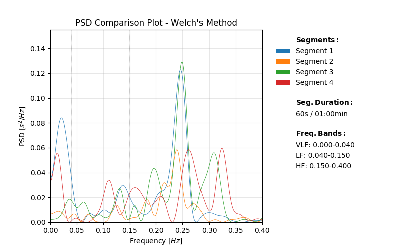
The plot of these examples should look like the following plot:

Comparison of PSDs computing the Welch’s method with default frequency bands.

If you want to specify custom frequency bands, define the limits in a Python dictionary as shown in the following example:

# Define custom frequency bands and add the ULF band
fbands = {'ulf': (0.0, 0.1), 'vlf': (0.1, 0.2), 'lf': (0.2, 0.3), 'hf': (0.3, 0.4)}

# Compute the PSDs with custom frequency bands
result = fd.psd_comparison(nni=nni, duration=60, method='welch', fbands=fbands)

You can also use the Autoregressive method and the Lomb-Scargle methods:

# Compute the PSDs and the comparison plot using the AR method and 60s segments
result = fd.psd_comparison(rpeaks=rpeaks, duration=60, method='ar')

# Compute the PSDs and the comparison plot using the Lomb-Scargle method and 60s segments
result = fd.psd_comparison(rpeaks=rpeaks, duration=60, method='lomb')

This should produce the following results:

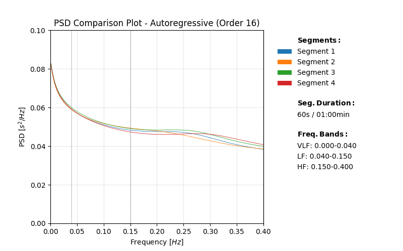
Comparison of PSDs computing the Autoregressive method with default frequency bands.

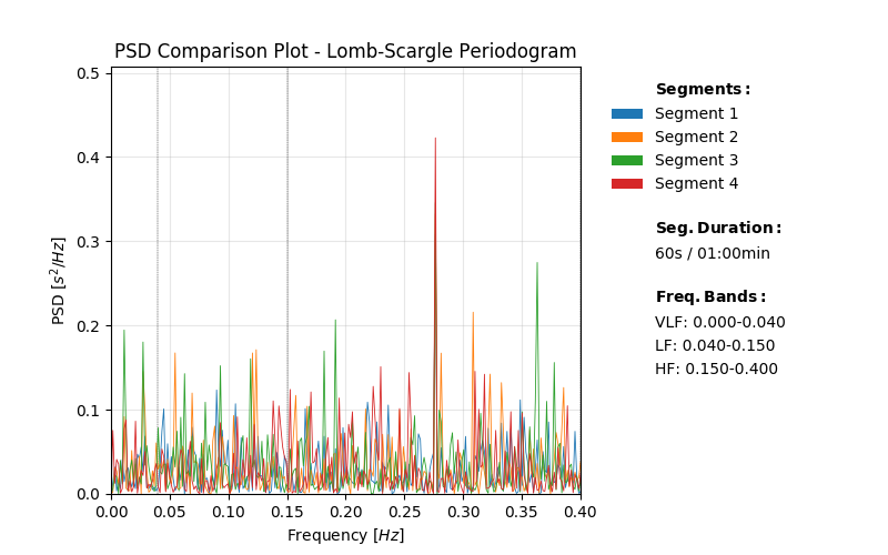
Comparison of PSDs computing the Lomb-Scargle method with default frequency bands.

Using the psd_comparison() function does not restrict you in specifying input parameters for the individual PSD methods. Define the compatible input parameters in Python dictionaries and pass them to the kwargs input dictionary of this function.

# Define input parameters for the 'welch_psd()' function & plot the PSD comparison
kwargs_welch = {'nfft': 2**8, 'detrend': False, 'window': 'hann'}
result = fd.psd_comparison(nni=nni, duration=60, method='welch', kwargs_method=kwargs_welch)

# Define input parameters for the 'lomb_psd()' function & plot the PSD comparison
kwargs_lomb = {'nfft': 2**8, 'ma_order': 5}
result = fd.psd_comparison(nni=nni, duration=60, method='lomb', kwargs_method=kwargs_lomb)

# Define input parameters for the 'ar_psd()' function & plot the PSD comparison
kwargs_ar = {'nfft': 2**8, 'order': 30}
result = fd.psd_comparison(nni=nni, duration=60, method='ar', kwargs_method=kwargs_ar)

Note

Some input parameters of the welch_psd(), ar_psd(), or lomb_psd() will be ignored when provided via the ‘kwargs_method’ input parameter to ensure the functionality this function

pyHRV is robust against invalid parameter keys. For example, if an invalid input parameter such as ‘threshold’ is provided, this parameter will be ignored and a warning message will be issued.

# Define custom input parameters using the kwargs dictionaries
kwargs_welch = {
   'nfft': 2**8,        # Valid key, will be used
   'threshold': 2**8    # Invalid key for the Welch's method domain, will be ignored
}

# Generate PSD comparison plot
result = fd.psd_comparison(nni=nni, duration=60, method='welch', kwargs_method=kwargs_welch)

This will trigger the following warning message.

Warning

Unknown kwargs for ‘welch_psd()’: threshold. These kwargs have no effect.

2.4.5. 3D PSD Waterfall Plot: psd_waterfall()¶

pyhrv.frequency_domain.psd_comparison(nni=None, rpeaks=None, segments=None, method='welch', fbands=None, kwargs_method={}, duration=300, show=True, legend=True)

Function Description

Computes a series of PSDs from NNI segments extracted from a NNI/R-Peak input series or a series of input NNI segments and plots the result in a single plot 3D plot. The PSDs are computed using the welch_psd(), lomb_psd(), or ar_psd() functions presented above.

This function aims to facilitate the visualization, comparison, and analyis of PSD evolution over time or NNI segments.

An example of a 3D waterfall plot generated by this function can be seen here:

Sample PSD comparison plot.

See also

Welch’s Method: welch_psd()
Lomb-Scargle Periodogram: lomb_psd()
Autoregressive Method: ar_psd()

If no frequency bands are specified, the default frequency band limits for the Very Low Frequency (VLF), Low Frequency (LF), and High Frequency (HF) bands as recommended by the HRV Guidelines are applied:

VLF: [0.00Hz - 0.04Hz]

LF: [0.04Hz - 0.15Hz]

HF: [0.15Hz - 0.40Hz]

Use the fbands parameter to specify custom frequency bands and the possibility to add the Ultra Low Frequency (ULF) band (see Application Notes & Examples & Tutorials below for more information).

The following parameters are computed from the PSDs and the specified frequency bands for each segment:

Peak frequencies [Hz]

Absolute powers [ms^2]

Relative powers [ms^2]

Logarithmic powers [log]

Normalized powers (LF & HF only)[-]

Total power of all frequency bands [ms^2]

Input Parameters

nni (array): NN intervals in [ms] or [s]
rpeaks (array): R-peak times in [ms] or [s]
segments (array of arrays): Array containing pre-selected segments for the PSD computation in [ms] or [s]
method (str): PSD estimation method (‘welch’, ‘ar’ or ‘lomb’)
fbands (dict, optional): Dictionary with frequency band specifications (default: None)
kwargs_method (dict): Dictionary of kwargs for the PSD computation functions ‘welch_psd()’, ‘ar_psd()’ or ‘lomb_psd()’
duration (int): Maximum duration duration per segment in [s] (default: 300s)
show (bool, optional): If True, show PSD plot figure (default: True)
legend (bool, optional): If True, add a legend with frequency bands to the plat (default: True)

Note

If fbands is none, the default values for the frequency bands will be set.

VLF: [0.00Hz - 0.04Hz]

LF: [0.04Hz - 0.15Hz]

HF: [0.15Hz - 0.40Hz]

See Application Notes & Examples & Tutorials below for more information on how to define custom frequency bands.

Returns (ReturnTuple Object)

The results of this function are returned in a nested biosppy.utils.ReturnTuple object with the following structure:

psd_waterfall_plot (matplotlib figure): Plot figure of the 3D waterfall plot

segN (dict): Plot data and PSD parameters of the segment N

The segN contains the Frequency Domain parameter results computed from the segment N. The segments have number keys (e.g. first segment = seg0, second segment = seg0, …, last segment = segN).

Example of a 2-segment output:

'seg0': {
        # Frequency Domain parameters of the first segment (e.g., 'fft_peak', 'fft_abs', 'fft_log', etc.)
}
'seg1': {
        # Frequency Domain parameters of the second segment (e.g., 'fft_peak', 'fft_abs', 'fft_log', etc.)
}
'psd_waterfall_plot': # matplotlib figure of the 3D waterfall plot

See also

The biosppy.utils.ReturnTuple Object

Important

If the the selected duration exceeds the overall duration of the input NNI series, the standard PSD plot and frequency domain results of the selected PDS method will be returned.

Keep an eye for warnings indicating if this is the case, as the output of this function will then provide the same output as the welch_psd(), lomb_psd() or ar_psd().

The kwargs_method input parameter will not have any effect in such cases.

Application Notes

It is not necessary to provide input data for nni and rpeaks. The parameter(s) of this function will be computed with any of the input data provided (nni or rpeaks). nni will be prioritized in case both are provided.

nni or rpeaks data provided in seconds [s] will automatically be converted to nni data in milliseconds [ms].

See also

Section NN Format: nn_format() for more information.

Incorrect frequency band specifications will be automatically corrected, if possible. For instance the following frequency bands contain overlapping frequency band limits which would cause issues when computing the frequency parameters:

fbands = {'vlf': (0.0, 0.25), 'lf': (0.2, 0.3), 'hf': (0.3, 0.4)}

Here, the upper band of the VLF band is greater than the lower band of the LF band. In this case, the overlapping frequency band limits will be switched:

fbands = {'vlf': (0.0, 0.2), 'lf': (0.25, 0.3), 'hf': (0.3, 0.4)}

Warning

Corrections of frequency bands trigger warnings which are displayed in the Python console. It is recommended to watch out for these warnings and to correct the frequency bands given that the corrected bands might not be optimal.

Important

This function generates matplotlib plot figures which, depending on the backend you are using, can interrupt your code from being executed whenever plot figures are shown. Switching the backend and turning on the matplotlib interactive mode can solve this behavior.

In case it does not - or if switching the backend is not possible - close all the plot figures to proceed with the execution of the rest your code after the plt.show().

See also

Examples & Tutorials

The following example code demonstrates how to use this function and how access the results stored in the biosppy.utils.ReturnTuple object.

You can use NNI series (nni) to compute the PSD comparison plot:

# Import packages
import pyhrv
import pyhrv.frequency_domain as fd

# Load NNI sample series
nni = pyhrv.utils.load_sample_nni()

# Compute the PSDs and the comparison plot using the Welch's method and 60s segments
result = fd.psd_waterfall(nni=nni, duration=60, method='welch')

# Access peak frequencies of the first segment using the key 'fft_peak'
print(result['psd_data']['seg1']['fft_peak'])

Alternatively, you can use R-peak series (rpeaks), too:

# Import packages
import biosppy
import pyhrv.frequency_domain as fd

# Load sample ECG signal
signal = np.loadtxt('./files/SampleECG.txt')[:, -1]

# Get R-peaks series using biosppy
t, filtered_signal, rpeaks = biosppy.signals.ecg.ecg(signal)[:3]

# Compute the PSDs and the comparison plot using the Welch's method and 60s segments
result = fd.psd_waterfall(rpeaks=rpeaks, duration=60, method='welch')

The plot of these examples should look like the following plot:

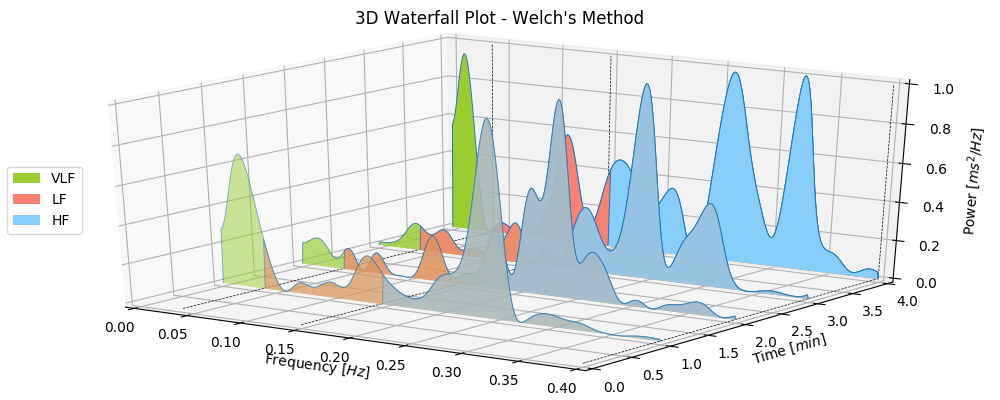
PSD waterfall computed using the Welch’s method with default frequency bands.

If you want to specify custom frequency bands, define the limits in a Python dictionary as shown in the following example:

# Define custom frequency bands and add the ULF band
fbands = {'ulf': (0.0, 0.1), 'vlf': (0.1, 0.2), 'lf': (0.2, 0.3), 'hf': (0.3, 0.4)}

# Compute the PSDs with custom frequency bands
result = fd.psd_waterfall(nni=nni, duration=60, method='welch', fbands=fbands)

You can also use the Autoregressive method and the Lomb-Scargle methods:

# Compute the PSDs and the waterfall plot using the AR method and 60s segments
result = fd.psd_waterfall(rpeaks=rpeaks, duration=60, method='ar')

# Compute the PSDs and the waterfall plot using the Lomb-Scargle method and 60s segments
result = fd.psd_waterfall(rpeaks=rpeaks, duration=60, method='lomb')

This should produce the following results:

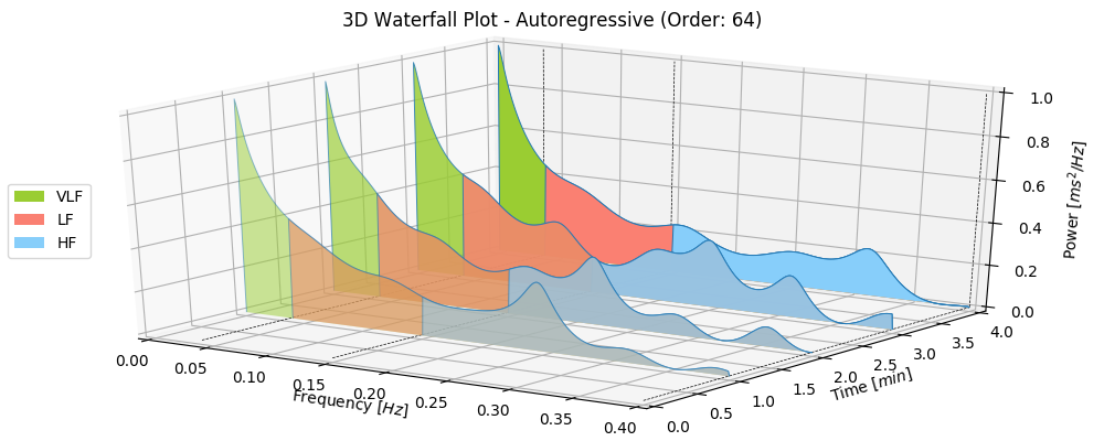
PSD waterfall computed using the Autoregressive method with default frequency bands.

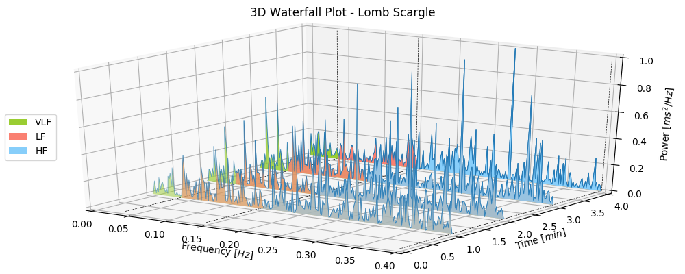
PSD waterfall computed using the Lomb-Scargle method with default frequency bands.

Using the psd_waterfall() function does not restrict you in specifying input parameters for the individual PSD methods. Define the compatible input parameters in Python dictionaries and pass them to the kwargs input dictionary of this function.

# Define input parameters for the 'welch_psd()' function & plot the PSD comparison
kwargs_welch = {'nfft': 2**8, 'detrend': False, 'window': 'hann'}
result = fd.psd_waterfall(nni=nni, duration=60, method='welch', kwargs_method=kwargs_welch)

# Define input parameters for the 'lomb_psd()' function & plot the PSD comparison
kwargs_lomb = {'nfft': 2**8, 'ma_order': 5}
result = fd.psd_waterfall(nni=nni, duration=60, method='lomb', kwargs_method=kwargs_lomb)

# Define input parameters for the 'ar_psd()' function & plot the PSD comparison
kwargs_ar = {'nfft': 2**8, 'order': 30}
result = fd.psd_waterfall(nni=nni, duration=60, method='ar', kwargs_method=kwargs_ar)

Note

Some input parameters of the welch_psd(), ar_psd(), or lomb_psd() will be ignored when provided via the ‘kwargs_method’ input parameter to ensure the functionality this function

pyHRV is robust against invalid parameter keys. For example, if an invalid input parameter such as ‘threshold’ is provided, this parameter will be ignored and a warning message will be issued.

# Define custom input parameters using the kwargs dictionaries
kwargs_welch = {
   'nfft': 2**8,        # Valid key, will be used
   'threshold': 2**8    # Invalid key for the Welch's method domain, will be ignored
}

# Generate PSD comparison plot
result = fd.psd_waterfall(nni=nni, duration=60, method='welch', kwargs=kwargs_welch)

This will trigger the following warning message.

Warning

Unknown kwargs for ‘welch_psd()’: threshold. These kwargs have no effect.

2.4.6. Domain Level Function: frequency_domain()¶

pyhrv.frequency_domain.frequency_domain(signal=None, nn=None, rpeaks=None, sampling_rate=1000., fbands=None, show=False, show_param=True, legend=True, kwargs_welch=None, kwargs_lomb=None, kwargs_ar=None)¶

Function Description

Computes PSDs using the Welch, Lomb, and Autoregressive methods by calling the welch_psd(), lomb_psd(), and ar_psd() functions, computes frequency domain parameters, and returns the results in a single biosppy.utils.ReturnTuple object.

See also

Welch’s Method: welch_psd()
Lomb-Scargle Periodogram: lomb_psd()
Autoregressive Method: ar_psd()

If no frequency bands are specified, the default frequency band limits for the Very Low Frequency (VLF), Low Frequency (LF), and High Frequency (HF) bands as recommended by the HRV Guidelines are applied:

VLF: [0.00Hz - 0.04Hz]

LF: [0.04Hz - 0.15Hz]

HF: [0.15Hz - 0.40Hz]

Use the fbands parameter to specify custom frequency bands and the possibility to add the Ultra Low Frequency (ULF) band (see Application Notes & Examples & Tutorials below for more information).

The following parameters are computed from the PSD and the specified frequency bands:

Peak frequencies [Hz]

Absolute powers [ms^2]

Relative powers [ms^2]

Logarithmic powers [log]

Normalized powers (LF & HF only)[-]

Total power of all frequency bands [ms^2]

Input Parameters

signal (array): ECG signal
nni (array): NN intervals in [ms] or [s]
rpeaks (array): R-peak times in [ms] or [s]
fbands (dict, optional): Dictionary with frequency band specifications (default: None)
show (bool, optional): If true, show all PSD plots.
show_param (bool, optional):
window (scipy.window function, optional): Window function used for PSD estimation (default: ‘hamming’)
show (bool, optional): If True, show PSD plot figure (default: True)
show_param (bool, optional): If true, list all computed parameters next to the plot (default: True)
kwargs_welch (dict, optional): Dictionary containing the kwargs for the ‘welch_psd’ function
kwargs_lomb (dict, optional): Dictionary containing the kwargs for the ‘lomb_psd’ function
kwargs_ar (dict, optional): Dictionary containing the kwargs for the ‘ar_psd’ function

Important

This function calls the PSD using either the signal, nni, or rpeaks data. Provide only one type of data, as it is not required to pass all three types at once.

Note

If fbands is none, the default values for the frequency bands will be set.

VLF: [0.00Hz - 0.04Hz]

LF: [0.04Hz - 0.15Hz]

HF: [0.15Hz - 0.40Hz]

See Application Notes & Examples & Tutorials below for more information on how to define custom frequency bands.

Returns (ReturnTuple Object) The results of this function are returned in a biosppy.utils.ReturnTuple object. This function returns the frequency parameters computed with all three PSD estimation methods. You can access all the parameters using the following keys (X = one of the methods ‘fft’, ‘ar’, ‘lomb’):

X_peak (tuple): Peak frequencies of all frequency bands [Hz]

X_abs (tuple): Absolute powers of all frequency bands [ms^2]

X_rel (tuple): Relative powers of all frequency bands [%]

X_log (tuple): Logarithmic powers of all frequency bands [log]

X_norm (tuple): Normalized powers of the LF and HF frequency bands [-]

X_ratio (float): LF/HF ratio [-]

X_total (float): Total power over all frequency bands [ms^2]

X_plot (matplotlib figure object): PSD plot figure object

fft_interpolation (str): Interpolation method used for NNI interpolation (hard-coded to ‘cubic’)

fft_resampling_frequency (int): Resampling frequency used for NNI interpolation [Hz] (hard-coded to 4Hz as recommended by the HRV Guidelines)

fft_window (str): Spectral window used for PSD estimation of the Welch’s method

lomb_ma (int): Moving average window size

ar_interpolation (str): Interpolation method used for NNI interpolation (hard-coded to ‘cubic’)

ar_resampling_frequency (int): Resampling frequency used for NNI interpolation [Hz] (hard-coded to 4Hz as recommended by the HRV Guidelines)

ar_order (int): Autoregressive model order

See also

The biosppy.utils.ReturnTuple Object

Application Notes

It is not necessary to provide input data for signal, nni and rpeaks. The parameter(s) of this function will be computed with any of the input data provided (signal, nni or rpeaks). The input data will be prioritized in the following order, in case multiple inputs are provided:

signal, 2. nni, 3. rpeaks.

nni or rpeaks data provided in seconds [s] will automatically be converted to nni data in milliseconds [ms].

See also

Section NN Format: nn_format() for more information.

Incorrect frequency band specifications will be automatically corrected, if possible. For instance the following frequency bands contain overlapping frequency band limits which would cause issues when computing the frequency parameters:

fbands = {'vlf': (0.0, 0.25), 'lf': (0.2, 0.3), 'hf': (0.3, 0.4)}

Here, the upper band of the VLF band is greater than the lower band of the LF band. In this case, the overlapping frequency band limits will be switched:

fbands = {'vlf': (0.0, 0.2), 'lf': (0.25, 0.3), 'hf': (0.3, 0.4)}

Warning

Corrections of frequency bands trigger warnings which are displayed in the Python console. It is recommended to watch out for these warnings and to correct the frequency bands given that the corrected bands might not be optimal.

This issue is shown in the following PSD plot where the corrected frequency bands above were used and there is no frequency band covering the range between 0.2Hz and 0.25Hz:

Welch PSD with corrected frequency bands and frequency band gaps.

Use the kwargs_welch dictionary to pass function specific parameters for the welch_psd() method. The following keys are supported:

nfft (int, optional): Number of points computed for the FFT result (default: 2**12)

detrend (bool, optional): If True, detrend NNI series by subtracting the mean NNI (default: True)

window (scipy.window function, optional): Window function used for PSD estimation (default: ‘hamming’)

Use the lomb_psd dictionary to pass function specific parameters for the lombg_psd() method. The following keys are supported:

nfft (int, optional): Number of points computed for the Lomb-Scargle result (default: 2**8)

ma_order (int, optional): Order of the moving average filter (default: None; no filter applied)

Use the ar_psd dictionary to pass function specific parameters for the ar_psd() method. The following keys are supported:

nfft (int, optional): Number of points computed for the FFT result (default: 2**12)

order (int, optional): Autoregressive model order (default: 16)

Important

The following input data is equally set for all the 3 methods using the input parameters of this function without using the kwargs dictionaries.

Defining these parameters/this specific input data individually in the kwargs dictionaries will have no effect:

nn (array): NN intervals in [ms] or [s]
rpeaks (array): R-peak times in [ms] or [s]
show (bool, optional): If True, show PSD plot figure (default: True)
fbands (dict, optional): Dictionary with frequency band specifications (default: None)
show_param (bool, optional): If true, list all computed PSD parameters next to the plot (default: True)
legend (bool, optional): If true, add a legend with frequency bands to the plot (default: True)

Any key or parameter in the kwargs dictionaries that is not listed above will have no effect on the functions.

Important

This function generates matplotlib plot figures which, depending on the backend you are using, can interrupt your code from being executed whenever plot figures are shown. Switching the backend and turning on the matplotlib interactive mode can solve this behavior.

In case it does not - or if switching the backend is not possible - close all the plot figures to proceed with the execution of the rest your code after the plt.show() function.

See also

Examples & Tutorials

The following example codes demonstrate how to use the frequency_domain() function.

You can choose either the ECG signal, the NNI series or the R-peaks as input data for the PSD estimation and parameter computation:

# Import packages
import biosppy
import pyhrv.frequency_domain as fd
import pyhrv.tools as tools

# Load sample ECG signal
signal = np.loadtxt('./files/SampleECG.txt')[:, -1]

# Get R-peaks series using biosppy
t, filtered_signal, rpeaks = biosppy.signals.ecg.ecg(signal)[:3]

# Compute NNI series
nni = tools.nn_intervals(t[rpeaks])

# OPTION 1: Compute PSDs using the ECG Signal
signal_results = fd.frequency_domain(signal=filtered_signal)

# OPTION 2: Compute PSDs using the R-peak series
rpeaks_results = fd.frequency_domain(rpeaks=t[rpeaks])

# OPTION 3: Compute PSDs using the
nni_results = fd.frequency_domain(nni=nni)

The output of all three options above will be the same.

Note

If an ECG signal is provided, the signal will be filtered and the R-peaks will be extracted using the biosppy.signals.ecg.ecg() function. Finally, the NNI series for the PSD estimation will be computed from the extracted R-peak series.

See also

biosppy.signals.ecg.ecg()

You can now access the frequency parameters of each method using the following commands:

# Access peak frequencies from each method (works the same for 'rpeaks_results' and 'nni_results')
print(signal_results['fft_peak'])
print(signal_results['lomb_peak'])
print(signal_results['ar_peak'])

The plots generated using the example above should look like the following plots:

Welch, Lomb-Scargle and Autoregressive PSDs with default parameters using only the frequency_domain() function.

If you want to specify custom frequency bands, define the limits in a Python dictionary as shown in the following example below:

Note

The frequency bands are equally defined for all three PSD estimation methods when using the frequency_domain() function. Use the individual method functions instead, in case you want to define method-specific frequency bands.

# Define custom frequency bands and add the ULF band
fbands = {'ulf': (0.0, 0.1), 'vlf': (0.1, 0.2), 'lf': (0.2, 0.3), 'hf': (0.3, 0.4)}

# Compute the PSD with custom frequency bands
result = fd.frequency_domain(nni, fbands=fbands)

The plots generated using the example above should look like the following plots:

Welch, Lomb-Scargle and Autoregressive PSDs with custom frequency bands using only the ``frequency_domain ()``function.

By default, the figure will contain the PSD plot on the left and the computed parameter results on the right side of the figure. Set the show_param to False if only the PSD is needed in the figure.

Using the frequency_domain() function does not restrict you in specifying input parameters for the individual PSD methods. Define the compatible input parameters in Python dictionaries and pass them to the kwargs input dictionaries of this function (see this functions Application Notes for a list of compatible parameters):

# Import packages
import biosppy
import pyhrv.frequency_domain as fd

# Load sample ECG signal
signal = np.loadtxt('./files/SampleECG.txt')[:, -1]

# Get R-peaks series using biosppy
t, filtered_signal, rpeaks = biosppy.signals.ecg.ecg(signal)[:3]

# Define input parameters for the 'welch_psd()' function
kwargs_welch = {'nfft': 2**8, 'detrend': False, 'window': 'hann'}

# Define input parameters for the 'lomb_psd()' function
kwargs_lomb = {'nfft': 2**8, 'ma_order': 5}

# Define input parameters for the 'ar_psd()' function
kwargs_ar = {'nfft': 2**8, 'order': 30}

# Compute PSDs using the ECG Signal
signal_results = fd.frequency_domain(signal=filtered_signal, show=True,
kwargs_welch=kwargs_lomb, kwargs_lomb=kwargs_lomb, kwargs_ar=kwargs_ar)

pyHRV is robust against invalid parameter keys. For example, if an invalid input parameter such as ‘threshold’ is provided in any of the frequency domain kwargs dictionaries, this parameter will be ignored and a warning message will

be issued.

# Define custom input parameters using the kwargs dictionaries
kwargs_welch = {
   'nfft': 2**8,        # Valid key, will be used
   'threshold': 2**8    # Invalid key for the Welch's method domain, will be ignored
}

# Compute HRV parameters
fd.frequency_domain(nni=nni, kwargs_welch=kwargs_welch)

This will trigger the following warning message.

Warning

Unknown kwargs for ‘welch_psd()’: threshold. These kwargs have no effect.

2.4.7. Frequency Parameters ¶

The following parameters and their computation formulas are computed from each of the PSD estimation methods computed using the welch_psd(), lomb_psd(), and ar_psd() functions presented above.

Note

The returned BioSPPy ReturnTuple object contains all frequency band parameters in parameter specific tuples of length 4 when using the ULF frequency band or of length 3 when NOT using the ULF frequency band. The structures of those tuples are shown in this example below:

Using ULF, VLF, LF and HF frequency bands:
fft_results['fft_peak'] = (ulf_peak, vlf_peak, lf_peak, hf_peak)
Using VLF, LF and HF frequency bands:
fft_results['fft_peak'] = (vlf_peak, lf_peak, hf_peak)

Absolute Powers

The absolute powers [ms^2] are individually computed for each frequency band as the sum of the power over the frequency band.

\[P_{abs} = \Delta f \sum_{f = f_{min}}^{f_{max}} S(f)\]

with:

\(P_{abs}\): Absolute power

\(\Delta f\): Frequency resolution

\(f_{min}\): Lower limit of the frequency band

\(f_{max}\): Upper limit of the frequency band

\(S(f)\): PSD function in dependence of the frequency \(f\)

The absolute powers are stored in the ReturnTuple object and can be accessed with one of the following keys depending on the PSD method being used:

fft_abs as a result of the welch_psd() function

lomb_abs as a result of the lomb_psd() function

ar_abs as a result of the ar_psd() function

Note

In case you are using the pyhrv.hrv() or the pyhrv.frequency_domain.frequency_domain() functions, you can use all the three keys listed above as all methods are computed using these functions.

Total Power

The total power [\(ms^2\)] of the PSD is computed as the sum of the absolute powers of all frequency bands:

\[P_{Total} = P_{ULF} + P_{VLF} + P_{LF} + P_{HF}\]

with:

\(P_{Total}\): Total power

\(P_{ULF}\): Absolute power of the ULF frequency band (= 0 if ULF is not specified)

\(P_{VLF}\): Absolute power of the VLF frequency band

\(P_{LF}\): Absolute power of the LF frequency band

\(P_{HF}\): Absolute power of the HF frequency band

The total power is stored in the ReturnTuple object and can be accessed with one of the following keys depending on the PSD method being used:

fft_total as a result of the welch_psd() function

lomb_total as a result of the lomb_psd() function

ar_total as a result of the ar_psd() function

Note

In case you are using the pyhrv.hrv() or the pyhrv.frequency_domain.frequency_domain() functions, you can use all the three keys listed above as all methods are computed using these functions.

Relative Power

The relative powers [\(a\)] are computed as the ratio between the absolute power of a frequency band and the total power:

\[P_{rel, z} = \frac{P_{abs,z}}{P_{Total}} * 100\]

with:

\(P_{rel, z}\): Relative power of the frequency band \(z\)

\(P_{abs, z}\): Absolute power of the frequency band \(z\)

\(z\): Frequency band (ULF, VLF, LF or HF)

\(P_{Total}\): Total power over all frequency bands

The relative powers are stored in the ReturnTuple object and can be accessed with one of the following key depending on the PSD method being used:

fft_rel as a result of the welch_psd() function

lomb_rel as a result of the lomb_psd() function

ar_rel as a result of the ar_psd() function

Note

In case you are using the pyhrv.hrv() or the pyhrv.frequency_domain.frequency_domain() functions, you can use all the three keys listed above as all methods are computed using these functions.

Logarithmic Powers

The logarithmic powers [\(log(ms^2)\)] are computed as follows total power:

\[P_{log, z} = log(P_{abs, z})\]

with:

\(P_{log, z}\): Logarithmic power of the frequency band \(z\)

\(P_{abs, z}\): Absolute power of the frequency band \(z\)

\(z\): Frequency band (ULF, VLF, LF or HF)

The logarithmic powers are stored in the ReturnTuple object and can be accessed with one of the following key depending on the PSD method being used:

fft_log as result of the welch_psd() function

lomb_log as result of the lomb_psd() function

ar_log as result of the ar_psd() function

Note

In case you are using the pyhrv.hrv() or the pyhrv.frequency_domain.frequency_domain() functions, you can use all the three keys listed above as all methods are computed using these functions.

Normalized Powers

The normalized powers [-] are computed for and based on the LF and HF frequency parameters only according to the following formulas:

\[P_{norm, LF} = \frac{P_{abs, LF}}{P_{abs, LF} + P_{abs, HF}} * 100\]

\[P_{norm, HF} = \frac{P_{abs, HF}}{P_{abs, LF} + P_{abs, HF}} * 100\]

with:

\(P_{norm, LF}\): Normalized power of the LF band

\(P_{abs, LF}\): Absolute power of the LF band

\(P_{norm, HF}\): Normalized power of the HF band

\(P_{abs, HF}\): Absolute power of the HF band

The normalized powers are stored in the ReturnTuple object and can be accessed with one of the following key depending on the PSD method being used:

fft_norm as result of the welch_psd() function

lomb_norm as result of the lomb_psd() function

ar_norm as result of the ar_psd() function

Note

Independently of the specified frequency band (with or without the VLF band) the results of this parameter are always returned in a 2-element tuple. The first element is the normalized power of the LF band with the second being the normalized power of the HF band.

fft_results['fft_norm'] = (lf_norm, hf_norm)

Note

In case you are using the pyhrv.hrv() or the pyhrv.frequency_domain.frequency_domain() functions, you can use all the three keys listed above as all methods are computed using these functions.

LF/HF Ratio

The LF/HF ratio is computed based on the absolute powers of the LF and HF bands:

\[\frac{LF}{HF} = \frac{P_{abs, LF}}{P_{abs, HF}}\]

with:

\(P_{abs, LF}\): Absolute power of the LF band

\(P_{abs, HF}\): Absolute power of the HF band

The LF/HF ratio is stored in the ReturnTuple object and can be accessed with one of the following keys depending on the PSD method being used:

fft_ratio (float) as result of the welch_psd() function

lomb_ratio (float) as result of the lomb_psd() function

ar_ratio (float) as result of the ar_psd() function

Note

Other than most of the other HRV frequency domain parameters, this parameter is always returned as a single float value rather than in a multi-dimensional tuple or array.

fft_results['fft_ratio'] = float(lf_hf_ratio)

Note

In case you are using the pyhrv.hrv() or the pyhrv.frequency_domain.frequency_domain() functions, you can use all the three keys listed above as all methods are computed using these functions.