2.5. Nonlinear Module ¶

The nonlinear.py module contains functions to compute nonlinear HRV parameters and methods.

See also

pyHRV Nonlinear Module source code

Module Contents

Nonlinear Module

See also

Useful links:

2.5.1. Poincaré: poincare()¶

pyhrv.nonlinear.poincare(nni=None, rpeaks=None, show=True, figsize=None, ellipse=True, vectors=True, legend=True, marker='o')¶

Function Description

Creates the Poincaré plot from a series of NN intervals or R-peak locations and derives the Poincaré related parameters SD1, SD2, SD2/SD1 ratio, and area of the Poincaré ellipse.

An example of the Poincaré scatter plot generated by this function can be seen here:

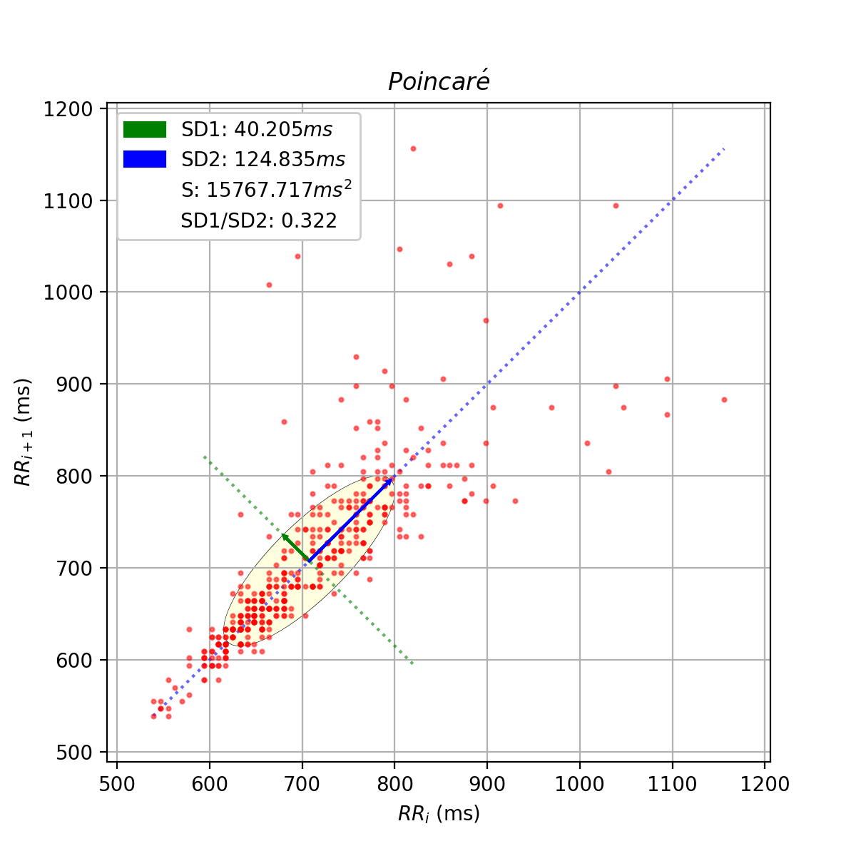
Poincaré scatter plot.

Input Parameters

nni (array): NN intervals in [ms] or [s].
rpeaks (array): R-peak times in [ms] or [s].
show (bool, optional): If True, show Poincaré plot (default: True)
figsize (array, optional): Matploltib figure size; Format: figisze=(width, height) (default: None: (6, 6)
ellipse (bool, optional): If True, shows fitted ellipse in plot (default: True)
vectors (bool, optional): If True, shows SD1 and SD2 vectors in plot (default: True)
legend (bool, optional): If True, adds legend to the Poincaré plot (default: True)
marker (str, optional): NNI marker in plot (must be compatible with the matplotlib markers (default: ‘o’)

Returns (ReturnTuple Object)

The results of this function are returned in a biosppy.utils.ReturnTuple object. Use the following keys below (on the left) to index the results:

poincare_plot (matploltib figure object): Poincaré plot figure

sd1 (float): Standard deviation (SD1) of the major axis

sd2 (float): Standard deviation (SD2) of the minor axis

sd_ratio (float): Ratio between SD1 and SD2 (SD2/SD1)

ellipse_area (float): Arrea S of the fitted ellipse

See also

The biosppy.utils.ReturnTuple Object

Computation

The SD1 parameter is the standard deviation of the data series along the minor axis and is computed using the SDSD parameter of the Time Domain.

\[SD1 = \sqrt{\frac{1}{2}SDSD^2}\]

with:

\(SD1\): Standard deviation along the minor axis

\(SDSD\): Standard deviation of successive differences (Time Domain parameter)

The SD2 parameter is the standard deviation of the data series along the major axis and is computed using the SDSD and the SDNN parameters of the Time Domain.

\[SD2 = \sqrt{2 SDNN^2 - \frac{1}{2} SDSD^2}\]

with:

\(SD2\): Standard deviation along the major axis

\(SDNN\): Standard deviation of the NNI series

\(SDSD\): Standard deviation of successive differences (Time Domain parameter)

The SD ratio is computed as

\[SD_{ratio} = \frac{SD2}{SD1}\]

The area of the ellipse fitted into the Poincaré scatter plot is computed as

\[S = \pi \cdot SD1 \cdot SD2\]

See also

Application Notes

It is not necessary to provide input data for nni and rpeaks. The parameter(s) of this function will be computed with any of the input data provided (nni or rpeaks). nni will be prioritized in case both are provided.

nni or rpeaks data provided in seconds [s] will automatically be converted to nni data in milliseconds [ms].

See also

Section NN Format: nn_format() for more information.

Use the ellipse and the vectors input parameters to hide the fitted ellipse and the SD1 and SD2 vectors from the Poincaré scatter plot.

Examples & Tutorials

The following example code demonstrates how to use this function and how to access the results stored in the returned biosppy.utils.ReturnTuple object.

You can use NNI series (nni) to compute the parameters:

# Import packages
import pyhrv
import pyhrv.nonlinear as nl

# Load sample data
nni = pyhrv.utils.load_sample_nni()

# Compute Poincaré using NNI series
results = nl.poincare(nni)

# Print SD1
print(results['sd1'])

The codes above create a plot similar to the plot below:

Poincaré scatter plot with default configurations.

Alternatively, you can use R-peak series (rpeaks):

# Import packages
import biosppy
import pyhrv.nonlinear as nl

# Load sample ECG signal
signal = np.loadtxt('./files/SampleECG.txt')[:, -1]

# Get R-peaks series using biosppy
t, _, rpeaks = biosppy.signals.ecg.ecg(signal)[:3]

# Compute Poincaré using R-peak series
results = pyhrv.nonlinear.poincare(rpeaks=t[rpeaks])

Use the ellipse, the vectors and the legend to show only the Poincaré scatter plot.

# Show the scatter plot without the fitted ellipse, the SD1 & SD2 vectors and the legend
results = nl.poincare(nni, ellipse=False, vectors=False, legend=False)

The generated plot is similar to the one below:

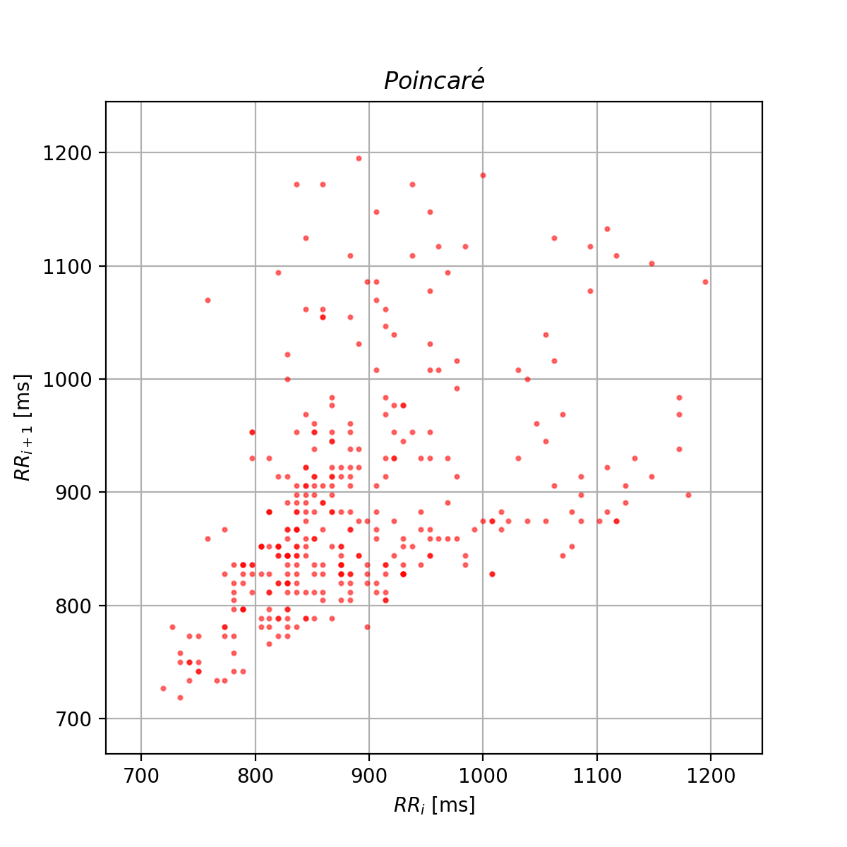
Barebone Poincaré scatter plot.

2.5.2. Sample Entropy: sample_entropy()¶

pyhrv.nonlinear.sampen(nni=None, rpeaks=None, dim=2, tolerance=None)¶

Function Description

Computes the sample entropy (sampen) of the NNI series for a given Entropy Embedding Dimension and vector distance tolerance.

Input Parameters

nni (array): NN intervals in [ms] or [s].
rpeaks (array): R-peak times in [ms] or [s].
dim (int, optional): Entropy embedding dimension (default: 2)
tolerance (int, float, optional): Tolerance distance for which the two vectors can be considered equal (default: std(NNI))

Returns (ReturnTuple Object)

The results of this function are returned in a biosppy.utils.ReturnTuple object. Use the following keys below (on the left) to index the results:

sample_entropy (float): Sample entropy of the NNI series.

See also

The biosppy.utils.ReturnTuple Object

Raises: TypeError: If tolerance is not a numeric value

Computation

This parameter is computed using the nolds.sampen() function.

See also

Nolds Documentation - Sampen

The default embedding dimension and tolerance values have been set to suitable HRV values.

Application Notes

It is not necessary to provide input data for nni and rpeaks. The parameter(s) of this function will be computed with any of the input data provided (nni or rpeaks). nni will be prioritized in case both are provided.

nni or rpeaks data provided in seconds [s] will automatically be converted to nni data in milliseconds [ms].

See also

Section NN Format: nn_format() for more information.

Examples & Tutorials

The following example code demonstrates how to use this function and how access the results stored in the returned biosppy.utils.ReturnTuple object.

You can use NNI series (nni) to compute the parameters:

# Import packages
import pyhrv
import pyhrv.nonlinear as nl

# Load sample data
nni = pyhrv.utils.load_sample_nni()

# Compute Sample Entropy using NNI series
results = nl.sampen(nni)

# Print Sample Entropy
print(results['sampen'])

Alternatively, you can use R-peak series (rpeaks):

# Import packages
import biosppy
import pyhrv.nonlinear as nl

# Load sample ECG signal
signal = np.loadtxt('./files/SampleECG.txt')[:, -1]

# Get R-peaks series using biosppy
t, _, rpeaks = biosppy.signals.ecg.ecg(signal)[:3]

# Compute Sample Entropy using R-peak series
results = nl.sampen(rpeaks=rpeaks)

2.5.3. Detrended Fluctuation Analysis: dfa()¶

pyhrv.nonlinear.dfa(nni=None, rpeaks=None, short=None, long=None, show=True, figsize=None, legend=False)¶

Function Description

Conducts Detrended Fluctuation Analysis (DFA) for short and long-term fluctuations of a NNI series.

An example plot of the DFA is shown below:

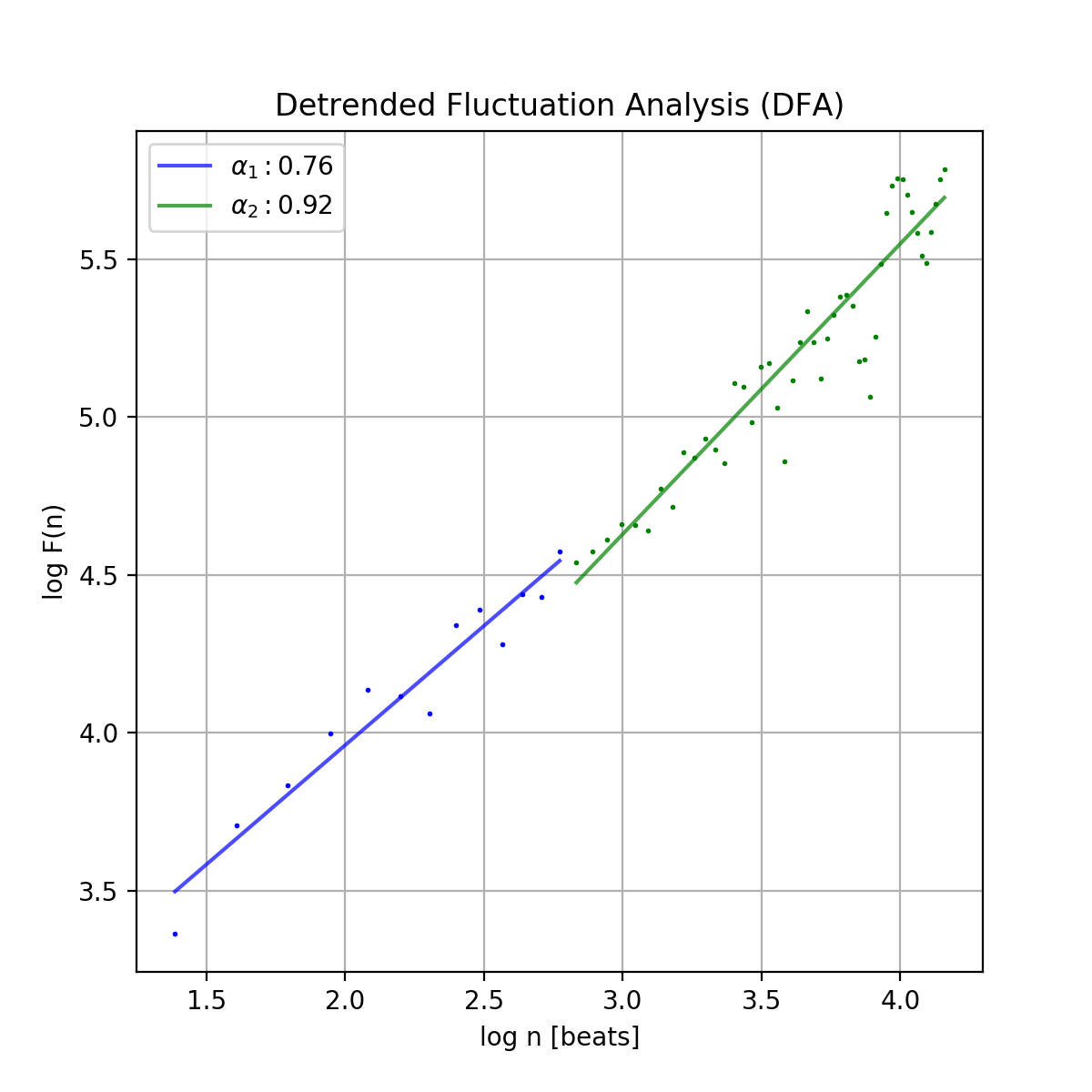
Detrended Fluctuation Analysis plot.

Input Parameters

nni (array): NN intervals in [ms] or [s].
rpeaks (array): R-peak times in [ms] or [s].
short (array, optional): Interval limits of the short-term fluctuations (default: None: [4, 16])
long (array, optional): Interval limits of the long-term fluctuations (default: None: [17, 64])
show (bool, optional): If True, shows DFA plot (default: True)
figsize (array, optional): 2-element array with the matplotlib figure size figsize. Format: figsize=(width, height) (default: will be set to (6, 6) if input is None).
legend (bool, optional): If True, adds legend with alpha1 and alpha2 values to the DFA plot (default: True)

Returns (ReturnTuple Object)

The results of this function are returned in a biosppy.utils.ReturnTuple object. Use the following keys below (on the left) to index the results:

dfa_short (float): Alpha value of the short-term fluctuations (alpha1)

dfa_long (float): Alpha value of the long-term fluctuations (alpha2)

See also

The biosppy.utils.ReturnTuple Object

Raises: TypeError: If tolerance is not a numeric value

Computation

This parameter is computed using the nolds.dfa() function.

See also

Nolds Documentation - DFA

The default short- and long-term fluctuation intervals have been set to HRV suitable intervals.

Application Notes

It is not necessary to provide input data for nni and rpeaks. The parameter(s) of this function will be computed with any of the input data provided (nni or rpeaks). nni will be prioritized in case both are provided.

nni or rpeaks data provided in seconds [s] will automatically be converted to nni data in milliseconds [ms].

See also

Section NN Format: nn_format() for more information.

The DFA cannot be computed if the number of NNI samples is lower than the specified short- and/or long-term fluctuation intervals. In this case, an empty plot with the information “Insufficient number of NNI samples for DFA” will be returned:

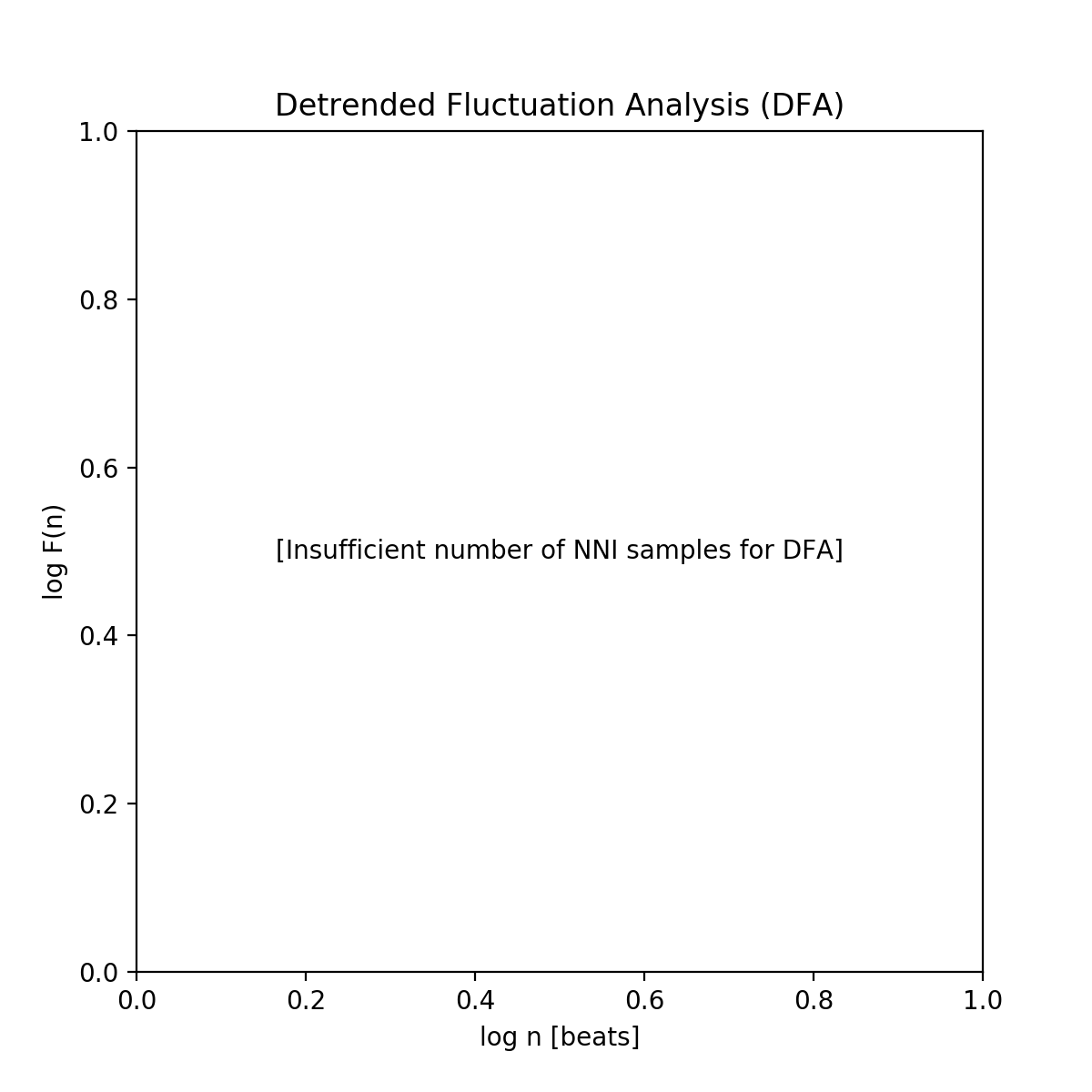
Resulting plot if there are not enough NNI samples for the DFA.

Important

This function generates matplotlib plot figures which, depending on the backend you are using, can interrupt your code from being executed whenever plot figures are shown. Switching the backend and turning on the matplotlib interactive mode can solve this behavior.

In case it does not - or if switching the backend is not possible - close all the plot figures to proceed with the execution of the rest your code after the plt.show() function.

See also

Examples & Tutorials

The following example code demonstrates how to use this function and how access the results stored in the returned biosppy.utils.ReturnTuple object.

You can use NNI series (nni) to compute the parameters:

# Import packages
import pyhrv
import pyhrv.nonlinear as nl

# Load sample data
nni = pyhrv.utils.load_sample_nni()

# Compute DFA using NNI series
results = nl.dfa(nni)

# Print DFA alpha values
print(results['dfa_short'])
print(results['dfa_long'])

Detrended Fluctuation Analysis plot.

Alternatively, you can use R-peak series (rpeaks):

# Import packages
import biosppy
import pyhrv.time_domain as td

# Load sample ECG signal
signal = np.loadtxt('./files/SampleECG.txt')[:, -1]

# Get R-peaks series using biosppy
t, _, rpeaks = biosppy.signals.ecg.ecg(signal)[:3]

# Compute DFA using R-peak series
results = nl.dfa(rpeaks=t[rpeaks])

2.5.4. Domain Level Function: nonlinear()¶

pyhrv.nonlinear.frequency_domain(nn=None, rpeaks=None, signal=None, sampling_rate=1000., show=False, kwargs_poincare={}, kwargs_sampen={}, kwargs_dfa{})¶

Function Description

Computes all the nonlinear HRV parameters of the Nonlinear module and returns them in a single ReturnTuple object.

See also

The individual parameter functions of this module for more detailed information about the computed parameters:

Poincaré: poincare()

Sample Entropy: sample_entropy()

Detrended Fluctuation Analysis: dfa()

Input Parameters

signal (array): ECG signal
nni (array): NN intervals in [ms] or [s]
rpeaks (array): R-peak times in [ms] or [s]
fbands (dict, optional): Dictionary with frequency band specifications (default: None)
show (bool, optional): If true, show all PSD plots.
kwargs_poincare (dict, optional): Dictionary containing the kwargs for the ‘poincare’ function
kwargs_sampen (dict, optional): Dictionary containing the kwargs for the ‘sample_entropy’ function
kwargs_dfa (dict, optional): Dictionary containing the kwargs for the ‘dfa’ function

Important

This function computes the nonlinear parameters using either the signal, nni, or rpeaks data. Provide only one type of data, as not all three types need to be passed as input argument

Returns (ReturnTuple Object) The results of this function are returned in a biosppy.utils.ReturnTuple object. This function returns the frequency parameters computed with all three PSD estimation methods. You can access all the parameters using the following keys (X = one of the methods ‘fft’, ‘ar’, ‘lomb’):

poincare_plot (matploltib figure object): Poincaré plot figure

sd1 (float): Standard deviation (SD1) of the major axis

sd2 (float): Standard deviation (SD2) of the minor axis

sd_ratio (float): Ratio between SD1 and SD2 (SD2/SD1)

ellipse_area (float): Arrea S of the fitted ellipse

sample_entropy (float): Sample entropy of the NNI series

dfa_short (float): Alpha value of the short-term fluctuations (alpha1)

dfa_long (float): Alpha value of the long-term fluctuations (alpha2)

See also

The biosppy.utils.ReturnTuple Object

Application Notes

It is not necessary to provide input data for signal, nni and rpeaks. The parameter(s) of this function will be computed with any of the input data provided (signal, nni or rpeaks). The input data will be prioritized in the following order, in case multiple inputs are provided:

signal, 2. nni, 3. rpeaks.

nni or rpeaks data provided in seconds [s] will automatically be converted to nni data in milliseconds [ms].

See also

Section NN Format: nn_format() for more information.

Use the kwargs_poincare dictionary to pass function specific parameters for the poincare() function. The following keys are supported:

ellipse (bool, optional): If True, shows fitted ellipse in plot (default: True)

vectors (bool, optional): If True, shows SD1 and SD2 vectors in plot (default: True)

legend (bool, optional): If True, adds legend to the Poincaré plot (default: True)

marker (str, optional): NNI marker in plot (must be compatible with the matplotlib markers (default: ‘o’)

Use the kwargs_sampen dictionary to pass function specific parameters for the sample_entropy() function. The following keys are supported:

dim (int, optional): Entropy embedding dimension (default: 2)

tolerance (int, float, optional): Tolerance distance for which the two vectors can be considered equal (default: std(NNI))

Use the kwargs_dfa dictionary to pass function specific parameters for the dfa() function. The following keys are supported:

short (array, optional): Interval limits of the short-term fluctuations (default: None: [4, 16])

long (array, optional): Interval limits of the long-term fluctuations (default: None: [17, 64])

legend (bool, optional): If True, adds legend to the Poincaré plot (default: True)

Important

The following input data is equally set for all the 3 methods using the input parameters of this function without using the kwargs dictionaries.

Defining these parameters/this specific input data individually in the kwargs dictionaries will have no effect:

show (bool, optional): If True, show Poincaré plot (default: True)
figsize (array, optional): Matploltib figure size; Format: figisze=(width, height) (default: None: (6, 6))

Any key or parameter in the kwargs dictionaries that is not listed above will have no effect on the functions.

Important

This function generates matplotlib plot figures which, depending on the backend you are using, can interrupt your code from being executed whenever plot figures are shown. Switching the backend and turning on the matplotlib interactive mode can solve this behavior.

In case it does not - or if switching the backend is not possible - close all the plot figures to proceed with the execution of the rest your code after the plt.show() function.

See also

Examples & Tutorials

The following example codes demonstrate how to use the nonlinear() function.

You can choose either the ECG signal, the NNI series or the R-peaks as input data for the PSD estimation and parameter computation:

# Import packages
import biosppy
import pyhrv.nonlinear as nl
import pyhrv.tools as tools

# Load sample ECG signal
signal = np.loadtxt('./files/SampleECG.txt')[:, -1]

# Get R-peaks series using biosppy
t, filtered_signal, rpeaks = biosppy.signals.ecg.ecg(signal)[:3]

# Compute NNI series
nni = tools.nn_intervals(t[rpeaks])

# OPTION 1: Compute using the ECG Signal
signal_results = nl.nonlinear(signal=filtered_signal)

# OPTION 2: Compute using the R-peak series
rpeaks_results = nl.nonlinear(rpeaks=t[rpeaks])

# OPTION 3: Compute using the
nni_results = nl.nonlinear(nni=nni)

The use of this function generates plots that are similar to the plots below:

Sample Poincaré scatter plot.

Sample Detrended Fluctuation Analysis plot.

Using the nonlinear() function does not limit you in specifying input parameters for the individual nonlinear functions. Define the compatible input parameters in Python dictionaries and pass them to the kwargs input dictionaries of this function (see this functions Application Notes for a list of compatible parameters):

# Import packages
import biosppy
import pyhrv.nonlinear as nl

# Load sample ECG signal
signal = np.loadtxt('./files/SampleECG.txt')[:, -1]

# Define input parameters for the 'poincare()' function
kwargs_poincare = {'ellipse': True, 'vectors': True, 'legend': True, 'markers': 'o'}

# Define input parameters for the 'sample_entropy()' function
kwargs_sampen = {'dim': 2, 'tolerance': 0.2}

# Define input parameters for the 'dfa()' function
kwargs_dfa = {'short': [4, 16] , 'long': [17, 64]}

# Compute PSDs using the ECG Signal
signal_results = fd.frequency_domain(signal=signal, show=True,
   kwargs_poincare=kwargs_poincare, kwargs_sampen=kwargs_sampen, kwargs_dfa=kwargs_dfa)

pyHRV is robust against invalid parameter keys. For example, if an invalid input parameter such as nfft is provided with the kwargs_poincare dictionary, this parameter will be ignored and a warning message will be issued.

# Define custom input parameters using the kwargs dictionaries
kwargs_poincare = {
   'ellipse': True,     # Valid key, will be used
   'nfft': 2**8         # Invalid key for the time domain, will be ignored
}

# Compute HRV parameters
nl.nonlinear(nni=nni, kwargs_poincare=kwargs_poincare)

This will trigger the following warning message.

Warning

Unknown kwargs for ‘poincare()’: nfft. These kwargs have no effect.

2.5. Nonlinear Module¶

2.5.1. Poincaré: poincare()¶

2.5.2. Sample Entropy: sample_entropy()¶

2.5.3. Detrended Fluctuation Analysis: dfa()¶

2.5.4. Domain Level Function: nonlinear()¶

2.5. Nonlinear Module ¶