2.6. Tools Module ¶

The Tools Module contains general purpose functions and key functionalities (e.g. computation of NNI series) for the entire HRV package, among other useful features for HRV analysis workflow (e.g. HRV export/import).

See also

pyHRV Tools Module source code

Module Contents

Tools Module

2.6.1. NN Intervals: nn_intervals()¶

pyhrv.tools.nn_intervals(rpeaks=None)¶

Function Description

Computes the series of NN intervals [ms] from a series of successive R-peak locations.

Input Parameters

rpeaks (array): R-peak times in [ms] or [s].

Returns

nni (array): Series of NN intervals in [ms].

Computation

The NN interval series is computed from the R-peak series as follows:

\[NNI_{j} = R_{j+1} - R_{j}\]

for \(0 <= j <= (n - 1)\)

with:

\(NNI_j\): NN interval j

\(R_j\): Current R-peak j

\(R_{j+1}\): Successive R-peak j+1

\(n\): Number of R-peaks

Application Notes

The nni series will be returned in [ms] format, even if the rpeaks are provided in [s] format.

See also

NN Format: nn_format() for more information about the [s] to [ms] conversion.

Example

The following example code demonstrates how to use this function:

# Import packages
import biosppy
import pyhrv.tools as tools

# Load sample ECG signal
signal = np.loadtxt('./files/SampleECG.txt')[:, -1]

# Get R-peaks series using biosppy
t, filtered_signal, rpeaks = biosppy.signals.ecg.ecg(signal)[:3]

# Compute NNI parameters
nni = tools.nn_intervals(t[rpeaks])

2.6.2. NN Interval Differences: nn_diff()¶

pyhrv.tools.nn_diff(nn=None)¶

Function Description

Computes the series of NN interval differences [ms] from a series of successive NN intervals.

Input Parameters

nni (array): NNI series in [ms] or [s].

Returns

nn_diff_ (array): Series of NN interval differences in [ms].

Computation

The NN interval series is computed from the R-peak series as follows:

\[\Delta NNI_j = NNI_{j+1} - NNI_j\]

for \(0 <= j <= (n - 1)\)

with:

\(\Delta NNI_j\): NN interval j

\(NNI_j\): Current NNI j

\(NNI_{j+1}\): Successive NNI j+1

\(n\): Number of NNI

Application Notes

The nn_diff_ series will be returned in [ms] format, even if the nni are provided in [s] format.

See also

NN Format: nn_format() for more information about the [s] to [ms] conversion.

Example

The following example code demonstrates how to use this function:

# Import packages
import biosppy
import pyhrv.tools as tools

# Load sample ECG signal
signal = np.loadtxt('./files/SampleECG.txt')[:, -1]

# Get R-peaks series using biosppy
t, filtered_signal, rpeaks = biosppy.signals.ecg.ecg(signal)[:3]

# Compute NNI parameters
nni = tools.nn_intervals(t[rpeaks])

# Compute NNI differences
delta_nni = tools.nn_diff(nni)

2.6.3. Heart Rate: heart_rate()¶

pyhrv.tools.heart_rate(nni=None, rpeaks=None)¶

Function Description

Computes a series of Heart Rate values in [bpm] from a series of NN intervals or R-peaks in [ms] or [s] or the HR from a single NNI.

Input Parameters

nni (int, float, array): NN interval series in [ms] or [s]
rpeaks (array): R-peak locations in [ms] or [s]

Returns

hr (array): Series of NN intervals in [ms].

Computation

The Heart Rate series is computed as follows:

\[HR_j = \frac{60000}{NNI_j}\]

for \(0 <= j <= n\)

with:

\(HR_j\): Heart rate j (in [bpm])

\(NNI_j\): NN interval j (in [ms])

\(n\): Number of NN intervals

Application Notes

The input nni series will be converted to [ms], even if the rpeaks are provided in [s] format.

See also

NN Format: nn_format() for more information about the [s] to [ms] conversion.

Example

The following example code demonstrates how to use this function:

# Import packages
import numpy as np
import pyhrv.tools as tools
import pyhrv.utils as utils

# Load sample data
nn = pyhrv.utils.load_sample_nni()

# Compute Heart Rate series
hr = tools.heart_rate(nn)

It is also possible to compute the HR from a single NNI:

# Compute Heart Rate from a single NNI
hr = tools.heart_rate(800)
# here: hr = 75 [bpm]

Attention

In this case, the input NNI must be provided in [ms] as the [s] to [ms] conversion is only conducted for series of NN Intervals.

2.6.4. Plot ECG: plot_ecg()¶

pyhrv.tools.plot_ecg(signal=None, t=None, samplin_rate=1000., interval=None, rpeaks=True, figsize=None, title=None, show=True)¶

Function Description

Plots ECG signal on a medical grade ECG paper-like figure layout.

An example of an ECG plot generated by this function can be seen here:

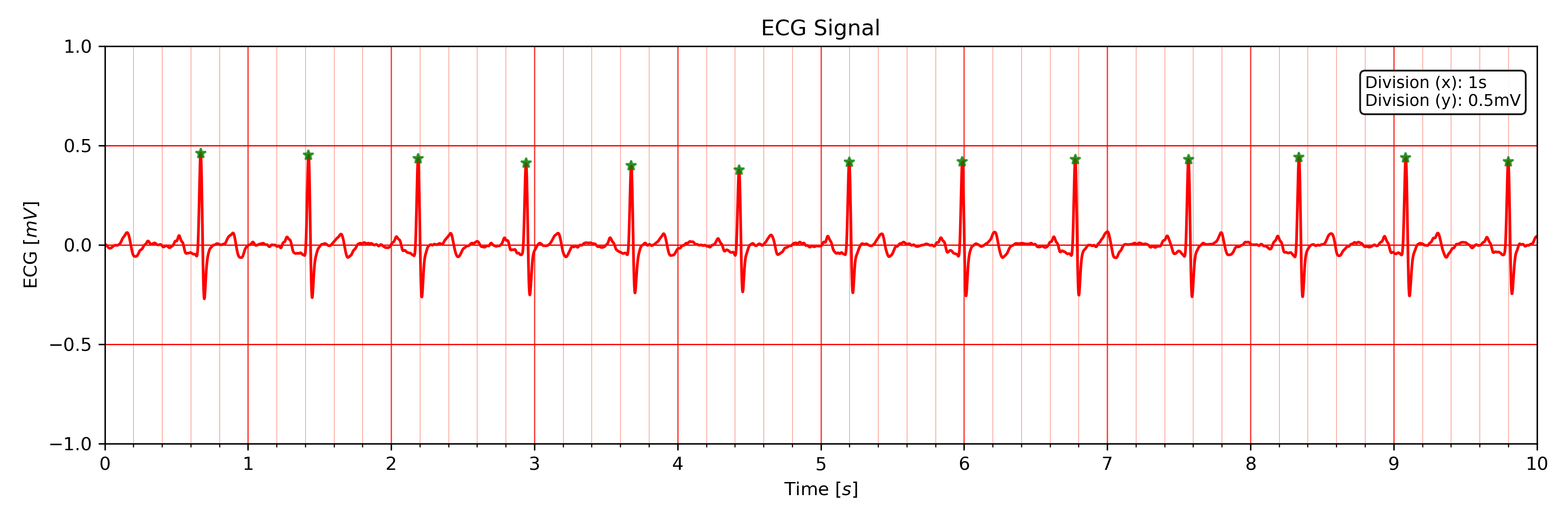
The x-Division does automatically adapt to the visualized interval (e.g., 10s interval -> 1s, 20s interval -> 2s, …).

Input Parameters

signal (array): ECG signal (filtered or unfiltered)
t (array, optional): Time vector for the ECG signal (default: None)
sampling_rate (int, float, optional): Sampling rate of the acquired signal in [Hz] (default: 1000Hz)
interval (array, optional): Visualization interval of the ECG signal plot (default: [0s, 10s])
rpeaks (bool, optional): If True, marks R-peaks in ECG signal (default: True)
figsize (array, optional): Matplotlib figure size (width, height) (default: None: (12, 4)
title (str, optional): Plot figure title (default: None)
show (bool, optional): If True, shows the ECG plot figure (default: True)

Returns

fig_ecg (matplotlib figure object): Matplotlibe figure of the ECG plot

Application Notes

The input nni series will be converted to [ms], even if nni are provided in [s] format.

See also

NN Format: nn_format() for more information about the [s] to [ms] conversion.

This functions marks, by default, the detected R-peaks. Use the rpeaks input parameter to turn on (rpeaks=True) or to turn of (rpeaks=False) the visualization of these markers.

Important

This parameter will have no effect if the number of R-peaks within the visualization interval is greater than 50. In this case, for reasons of plot clarity, no R-peak markers will be added to the plot.

The time axis scaling will change depending on the duration of the visualized interval:

t in [s] if visualized duration <= 60s

t in [mm:ss] (minutes:seconds) if 60s < visualized duration <= 1h

t in [hh:mm:ss] (hours:minutes:seconds) if visualized duration > 1h

Example

# Import
import pyhrv.tools as tools

# Load sample ECG signal
signal = np.loadtxt('./files/SampleECG.txt')[:, -1]

# Plot ECG
tools.plot_ecg(signal)

The plot of this example should look like the following plot:

Default visualization interval of the plot_ecg() function.

Use the interval input parameter to change the visualization interval using a 2-element array ([lower_interval_limit, upper_interval_limit]; default: 0s to 10s). Additionally, use the rpeaks parameter to toggle the R-peak markers.

The following code sets the visualization interval from 0s to 20s and hides the R-peak markers:

# Plot ECG
tools.plot_ecg(signal, interval=[0, 20], rpeaks=False)

The plot of this example should look like the following plot:

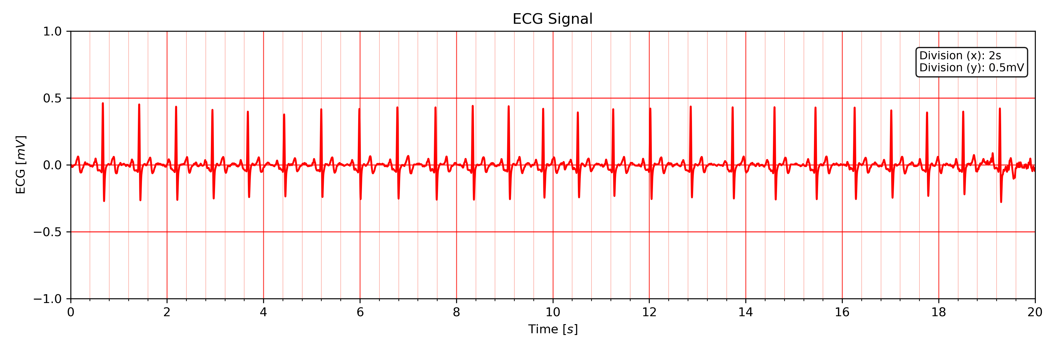
Visualizing the first 20 seconds of the ECG signal without R-peak markers.

Use the title input parameter to add titles to the ECG plot:

# Plot ECG
tools.plot_ecg(signal, interval=[0, 20], rpeaks=False, title='This is a Title')

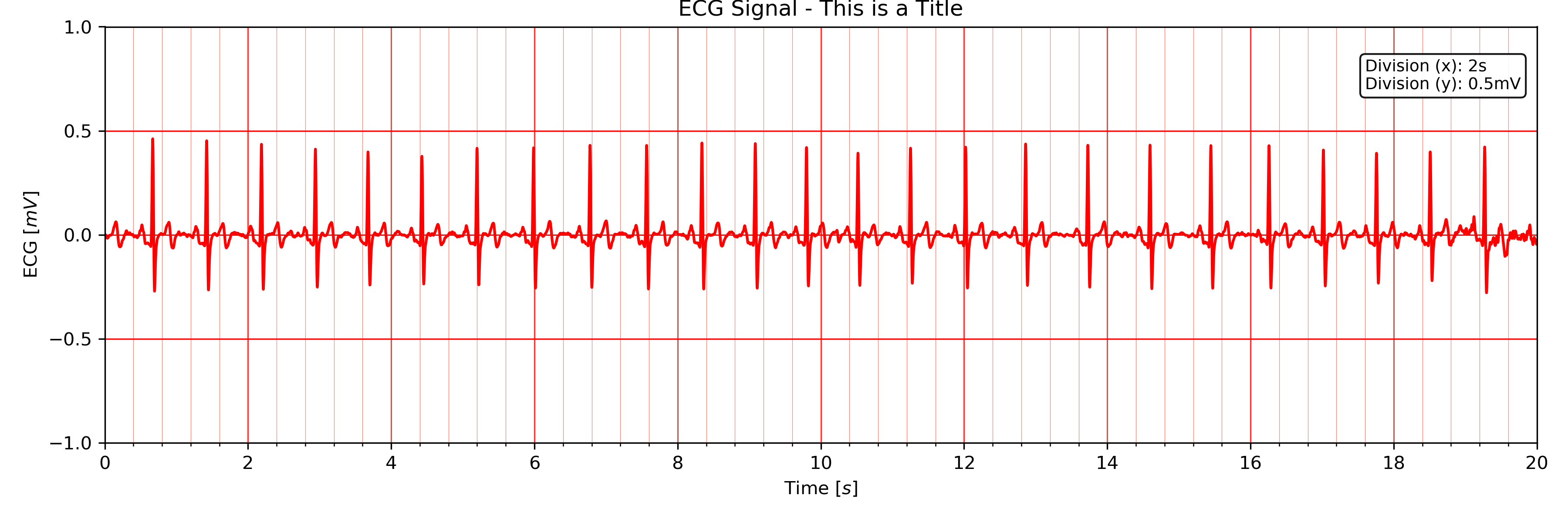
ECG plot with custom title.

2.6.5. Tachogram: tachogram()¶

pyhrv.tools.tachogram(signal=None, nn=None, rpeaks=None, sampling_rate=1000., hr=True, interval=None, title=None, figsize=None, show=True)¶

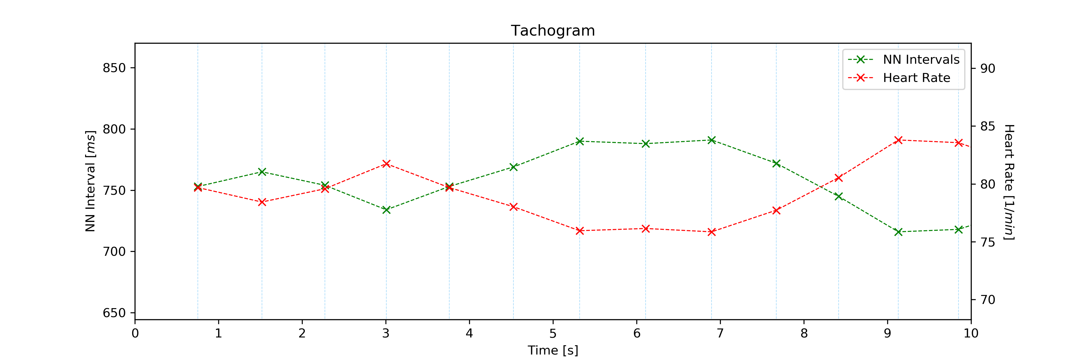
Function Description

Plots Tachogram (NNI & HR) of an ECG signal, NNI or R-peak series.

An example of a Tachogram plot generated by this function can be seen here:

Input Parameters

signal (array): ECG signal (filtered or unfiltered)
nni (array): NN interval series in [ms] or [s]
rpeaks (array): R-peak locations in [ms] or [s] - t (array, optional): Time vector for the ECG signal (default: None)
sampling_rate (int, optional): Sampling rate in [hz] of the ECG signal (default: 1000Hz)
hr (bool, optional): If True, plot HR seres in [bpm] on second axis (default: True)
interval (array, optional): Visualization interval of the Tachogram plot (default: None: [0s, 10s])
title (str, optional): Optional plot figure title (default: None)
figsize (array, optional): Matplotlib figure size (width, height) (default: None: (12, 4))
show (bool, optional): If True, shows the ECG plot figure (default: True)

Returns

fig (matplotlib figure object): Matplotlib figure of the Tachogram plot.

Application Notes

The input nni series will be converted to [ms], even if the rpeaks or nni are provided in [s] format.

See also

NN Format: nn_format() for more information about the [s] to [ms] conversion.

Example

The following example demonstrates how to load an ECG signal.

# Import
import pyhrv.tools as tools

# Load sample ECG signal
signal = np.loadtxt('./files/SampleECG.txt')[:, -1]

# Plot Tachogram
tools.tachogram(signal)

Alternatively, use R-peak data to plot the histogram…

# Import
import biosppy
import pyhrv.tools as tools

# Load sample ECG signal
signal = np.loadtxt('./files/SampleECG.txt')[:, -1]

# Get R-peaks series using biosppy
t, filtered_signal, rpeaks = biosppy.signals.ecg.ecg(signal)[:3]
# Plot Tachogram
tools.tachogram(rpeaks=t[rpeaks])

… or using directly the NNI series…

# Compute NNI intervals from the R-peaks
nni = tools.nn_intervals(t[rpeaks])

# Plot Tachogram
tools.tachogram(nni=nni)

The plots generated by the examples above should look like the plot below:

Tachogram with default visualization interval.

Use the interval input parameter to change the visualization interval (default: 0s to 10s; here: 0s to 20s):

# Plot ECG
tools.tachogram(signal=signal, interval=[0, 20])

The plot of this example should look like the following plot:

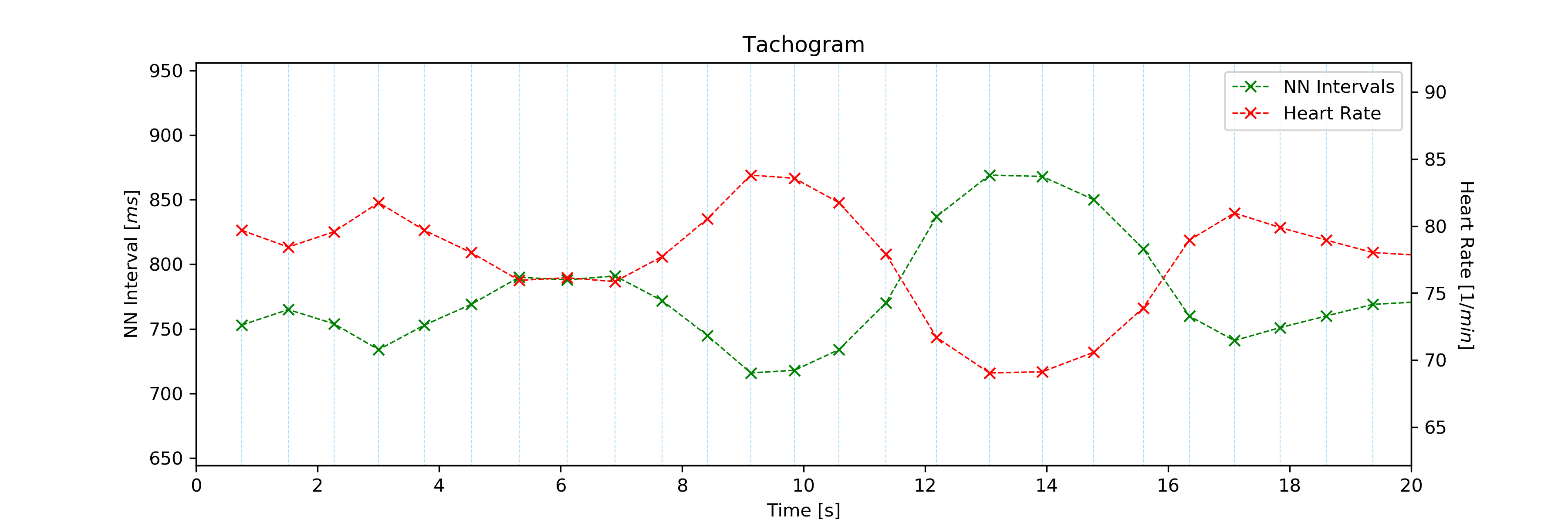
Tachogram with custom visualization interval.

Note

Interval limits which are out of bounce will automatically be corrected.

Example:

lower limit < 0 -> lower limit = 0
upper limit > maximum ECG signal duration -> upper limit = maximum ECG signal duration

Set the hr parameter to False in case only the NNI Tachogram is needed:

# Plot ECG
tools.tachogram(signal=signal, interval=[0, 20], hr=False)

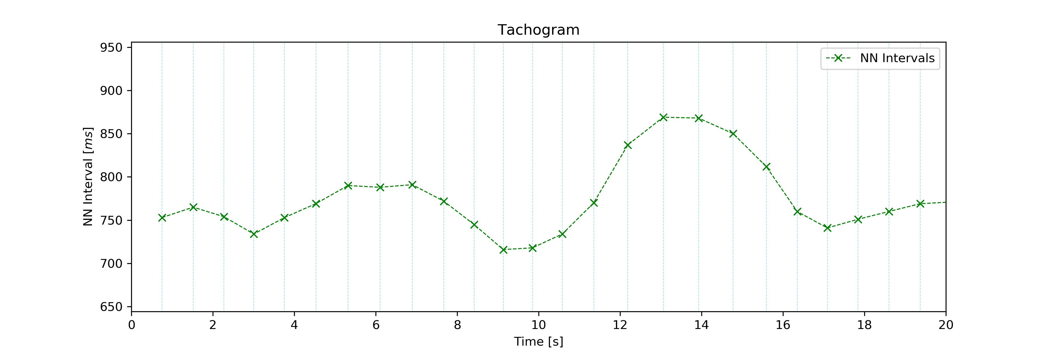
Tachogram of the NNI series only.

The time axis scaling will change depending on the duration of the visualized interval:

t in [s] if visualized duration <= 60s

t in [mm:ss] (minutes:seconds) if 60s < visualized duration <= 1h

t in [hh:mm:ss] (hours:minutes:seconds) if visualized duration > 1h

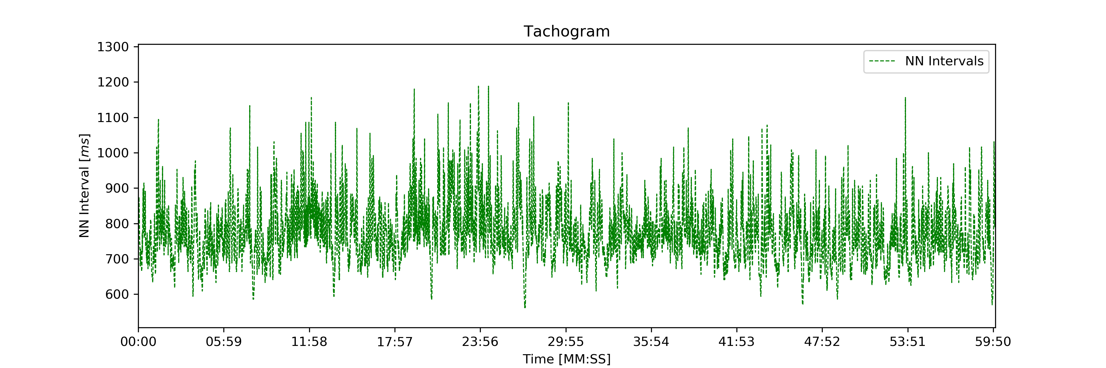
Tachogram of an ~1h NNI series.

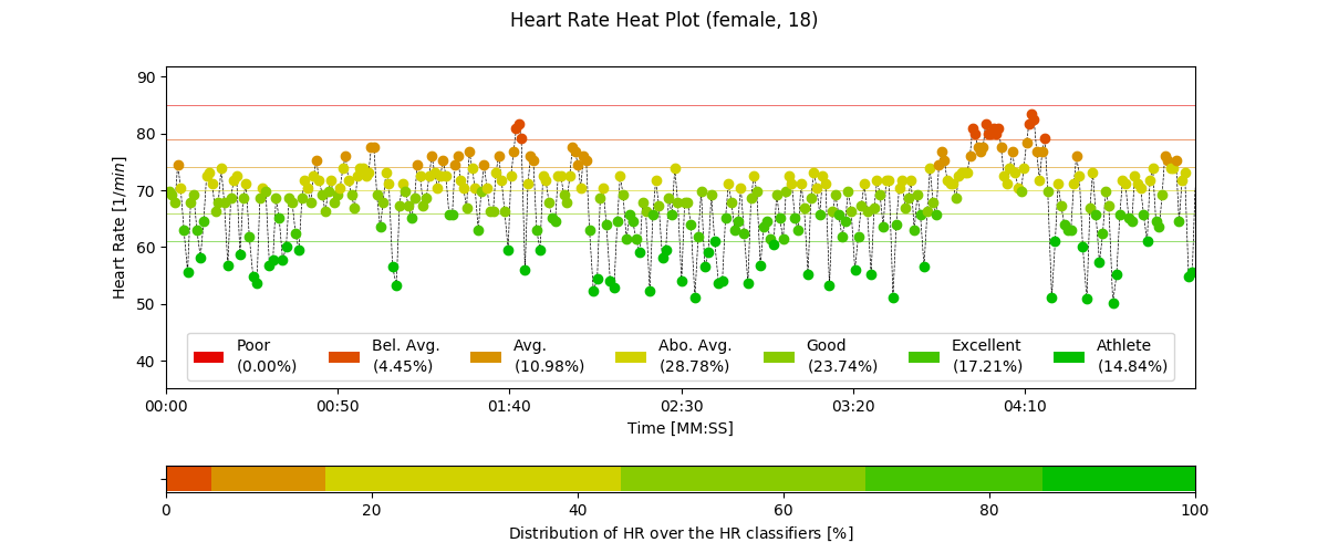
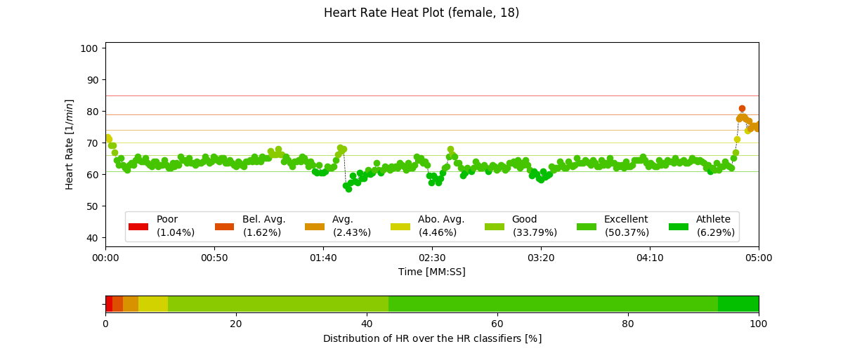
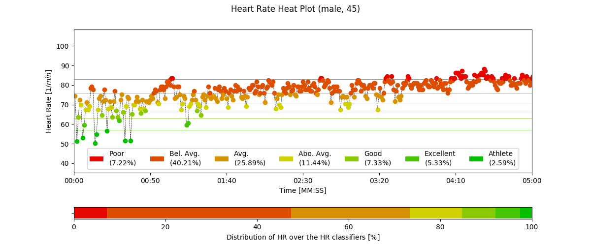
2.6.6. Heart Rate Heatplot: hr_heatplot()¶

pyhrv.tools.hr_heatplot(signal=None, nn=None, rpeaks=None, sampling_rate=1000., hr=True, interval=None, title=None, figsize=None, show=True)¶

Function Description

Graphical visualization & classification of HR performance based on normal HR ranges by age and gender.

An example of a Heart Rate Heatplot generated by this function can be seen here:

Input Parameters

nni (array): NN interval series in [ms] or [s]
rpeaks (array): R-peak locations in [ms] or [s] - t (array, optional): Time vector for the ECG signal (default: None)
signal (array): ECG signal (filtered or unfiltered)
sampling_rate (int, optional): Sampling rate in [hz] of the ECG signal (default: 1000Hz)
age (int, float): Age of the subject (default: 18)
gender (str): Gender of the subject (‘m’, ‘male’, ‘f’, ‘female’; default: ‘male’)
interval (list, optional): Sets visualization interval of the signal (default: [0, 10])
figsize (array, optional): Matplotlib figure size (weight, height) (default: (12, 4))
show (bool, optional): If True, shows plot figure (default: True)

Returns

The results of this function are returned in a biosppy.utils.ReturnTuple object. Use the following keys below (on the left) to index the results:

hr_heatplot (matplotlib figure object): Matplotlib figure of the Heart Rate Heatplot.

Application Notes

The input nni series will be converted to [ms], even if the rpeaks or nni are provided in [s] format.

See also

NN Format: nn_format() for more information about the [s] to [ms] conversion.

Interval limits which are out of bounce will automatically be corrected:

lower limit < 0 -> lower limit = 0

upper limit > maximum ECG signal duration -> upper limit = maximum ECG signal duration

The time axis scaling will change depending on the duration of the visualized interval:

t in [s] if visualized duration <= 60s

t in [mm:ss] (minutes:seconds) if 60s < visualized duration <= 1h

t in [hh:mm:ss] (hours:minutes:seconds) if visualized duration > 1h

Example

The following example demonstrates how to load an ECG signal.

# Import
import pyhrv.tools as tools

# Load sample ECG signal
signal = np.loadtxt('./files/SampleECG.txt')[:, -1]

# Plot Heart Rate Heatplot using an ECG signal
tools.hr_heatplot(signal=signal)

Alternatively, use R-peak or NNI data to plot the HR Heatplot…

# Import
import biosppy
import pyhrv.tools as tools

# Load sample ECG signal
signal = np.loadtxt('./files/SampleECG.txt')[:, -1]

# Get R-peaks series using biosppy
t, filtered_signal, rpeaks = biosppy.signals.ecg.ecg(signal)[:3]

tools.hr_heatplot(rpeaks=t[rpeaks])

… or using directly the NNI series…

# Compute NNI intervals from the R-peaks
nni = tools.nn_intervals(t[rpeaks])

# Plot HR Heatplot using the NNIs
tools.hr_heatplot(signal=signal)

The following plots are example results of this function:

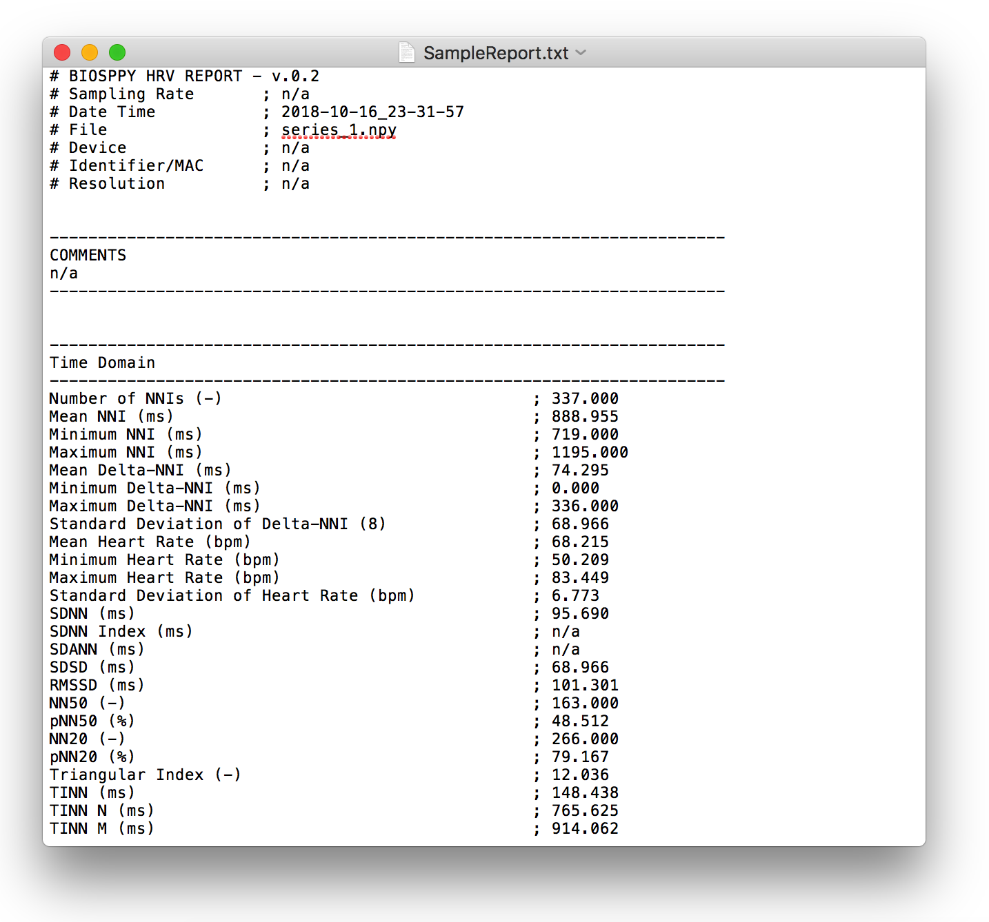
2.6.7. HRV Reports: hrv_report()¶

pyhrv.tools.hrv_report(results=None, path=None, rfile=None, nn=None, info={}, file_format='txt', delimiter=';', hide=False, plots=False)¶

Function Description

Generates HRV report (in .txt or .csv format) of the provided HRV results. You can find a sample report generated with this function here.

Input Parameters

results (dict, ReturnTuple object): Computed HRV parameter results
path (str): Absolute path of the output directory
rfile (str): Output file name
nni (array, optional): NN interval series in [ms] or [s]
info (dict, optional): Dictionary with HRV metadata
file_format (str, optional): Output file format, select ‘txt’ or ‘csv’ (default: ‘txt’)
delimiter (str, optional): Delimiter separating the columns in the report (default: ‘;’)
hide (bool, optional): Hide parameters in report that have not been computed
plots (bool, optional): If True, save plot figures in .png format

Note

The info dictionary can contain the following metadata:

key: file - Name of the signal acquisition file

key: device - ECG acquisition device

key: identifier - ECG acquisition device identifier (e.g. MAC address)

key: fs - Sampling rate used during ECG acquisition

key: resolution - Resolution used during acquisition

Any other key will be ignored.

Important

It is recommended to use absolute file paths when using the path parameter to ensure the correct functionality of this function.

Raises

TypeError: If no HRV results are provided
TypeError: If no file or directory path is provided
TypeError: If the specified selected file format is not supported
IOError: If the selected output file or directory does not exist

Application Notes

This function uses the weak _check_fname() function found in this module to prevent the (accidental) overwriting of existing HRV reports. If a file with the file name rfile does exist in the specified path, then the file name will be incremented.

For instance, if a report file with the name SampleReport.txt exists, this file will not be overwritten, instead, the file name of the new report will be incremented to SampleReport_1.txt.

If the file with the file name SampleReport_1.txt exists, the file name of the new report will be incremented to SampleReport_2.txt, and so on…

Important

The maximum supported number of file name increments is limited to 999 files, i.e., using the example above, the implemented file protection mechanisms will go up to SampleReport_999.txt.

If no file name is provided, an automatic file name with a time stamp will be generated for the generated report (hrv_report_YYYY-MM-DD_hh-mm-ss.txt or hrv_report_YYYY-MM-DD_hh-mm-ss.txt).

Example

The following example code demonstrates how to use this function:

# Import packages
import pyhrv
import numpy as np

# Load Sample NNI series (~5min)
nni = pyhrv.utils.load_sample_nni()

# Compute HRV results
results = pyhrv.hrv(nn=nni)

# Create HRV Report
pyhrv.tools.hrv_report(results, rfile='SampleReport', path='/my/favorite/path/')

This generates a report looking like the one below:

See also

2.6.8. HRV Export: hrv_export()¶

pyhrv.tools.hrv_export(results=None, path=None, efile=None, comment=None, plots=False)¶

Function Description

Exports HRV results into a JSON file. You can find a sample export generated with this function here.

Input Parameters

results (dict, ReturnTuple object): Computed HRV parameter results
path (str): Absolute path of the output directory
efile (str): Output file name
comment (str, optional): Optional comment
plots (bool, optional): If True, save figures of the results in .png format

Important

It is recommended to use absolute file paths when using the path parameter to ensure the correct operation of this function.

Returns

efile (str): Absolute path of the output report file (may vary from the input data)

Raises

TypeError: If no HRV results are provided
TypeError: If no file or directory path is provided
TypeError: If specified selected file format is not supported
IOError: If the selected output file or directory does not exist

Application Notes

This function uses the weak _check_fname() function found in this module to prevent the (accidental) overwriting of existing HRV exports. If a file with the file name efile exists in the specified path, then the file name will be incremented.

For instance, if an export file with the name SampleExport.json exists, this file will not be overwritten, instead, the file name of the new export file will be incremented to SampleExport_1.json.

If the file with the file name SampleExport_1.json exists, the file name of the new export will be incremented to SampleExport_2.json, and so on.

Important

The maximum supported number of file name increments is limited to 999 files, i.e., using the example above, the implemented file protection mechanisms will go up to SampleExport_999.json.

If no file name is provided, an automatic file name with a time stamp will be generated for the generated report (hrv_export_YYYY-MM-DD_hh-mm-ss.json).

Example

The following example code demonstrates how to use this function:

# Import packages
import pyhrv
import numpy as np
import pyhrv.tools as tools

# Load Sample NNI series (~5min)
nni = np.load('series_1.npy')

# Compute HRV results
results = pyhrv.hrv(nn=nni)

# Export HRV results
tools.hrv_export(results, efile='SampleExport', path='/my/favorite/path/')

See also

Sample HRV export

2.6.9. HRV Import: hrv_import()¶

pyhrv.tools.hrv_import(hrv_file=None)¶

Function Description

Imports HRV results stored in JSON files generated with the ‘hrv_export()’.

See also

HRV Export: hrv_export() function
Sample HRV export

Input Parameters

hrv_file (str, file handler): File handler or absolute string path of the HRV JSON file

Returns

output (ReturnTuple object): All HRV parameters stored in a biosppy.utils.ReturnTuple object

Raises

TypeError: If no file path or handler is provided

Example

The following example code demonstrates how to use this function:

# Import packages
import pyhrv.tools as tools

# Import HRV results
hrv_results = tools.hrv_import('/path/to/my/HRVResults.json')

See also

HRV keys file for a full list of HRV parameters and their respective keys.

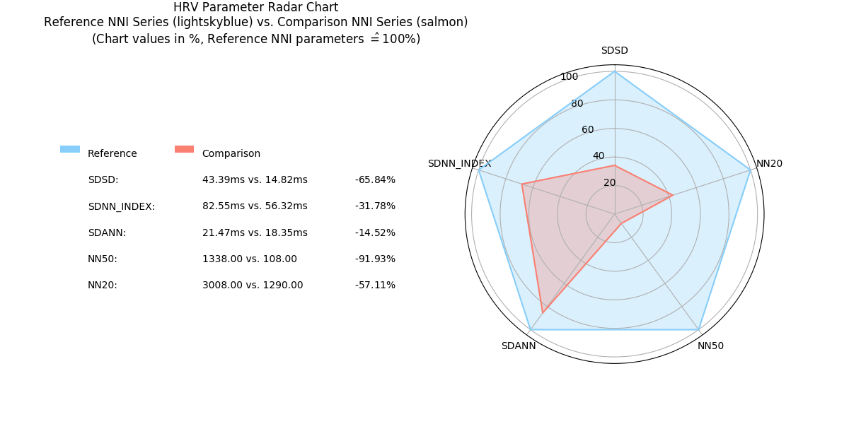
2.6.10. Radar Chart: radar_chart()¶

pyhrv.tools.radar_chart(nni=None, rpeaks=None, comparison_nni=None, comparison_rpeaks=None, parameters=None, reference_label='Reference', comparison_label='Comparison', show=True, legend=Tre)¶

Function Description

Plots a radar chart of HRV parameters to visualize the evolution the parameters computed from a NNI series (e.g. extracted from an ECG recording while doing sports) compared to a reference/baseline NNI series (e.g. extracted from an ECG recording while at rest).

The radarchart normalizes the values of the reference NNI series with the values extracted from the baseline NNI this series being used as the 100% reference values.

Example:

Reference NNI series: SDNN = 100ms → 100%
Comparison NNI series: SDNN = 150ms → 150%

The radar chart is not limited by the number of HRV parameters to be included in the chart; it dynamically adjusts itself to the number of compared parameters.

An example of a Radar Chart plot generated by this function can be seen here:

Input Parameters

nni (array): NN interval series in [ms] or [s] (default: None)
rpeaks (array): R-peak locations in [ms] or [s] (default: None)
comparison_nni (array): Comparison NNI series in [ms] or [s] (default: None)
comparison_rpeaks (array): Comparison R-peak series in [ms] or [s] (default: None)
parameters (list): List of pyHRV parameters (see hrv_keys.json file for a full list of available parameters)
reference_label (str, optional): Plot label of the reference input data (e.g. ‘ECG while at rest’; default: ‘Reference’)
comparison_label (str, optional): Plot label of the comparison input data (e.g. ‘ECG while running’; default: ‘Comparison’)
show (bool, optional): If True, shows plot figure (default: True).
legend (bool, optional): If true, add a legend with the computed results to the plot (default: True)

Returns (ReturnTuple Object)

The results of this function are returned in a biosppy.utils.ReturnTuple object. Use the following key below (on the left) to index the results:

reference_results (dict): HRV parameters computed from the reference input data

comparison_results (dict): HRV parameters computed from the comparison input data

radar_plot (dict): Resulting radar chart plot figure

Raises

TypeError: If an error occurred during the computation of a parameter
TypeError: If no input data is provided for the baseline/reference NNI or R-Peak series
TypeError: If no input data is provided for the comparison NNI or R-Peak series
TypeError: If no selection of pyHRV parameters is provided
ValueError: If less than 2 pyHRV parameters were provided

Application Notes

The input nni series will be converted to [ms], even if the rpeaks or nni are provided in [s] format.

See also

NN Format: nn_format() for more information about the [s] to [ms] conversion.

It is not necessary to provide input data for nni and rpeaks. The parameter(s) of this function will be computed with any of the input data provided (nni or rpeaks). nni will be prioritized in case both are provided. This is both valid for the reference as for the comparison input series.

Example

The following example shows how to compute the radar chart from two NNI series (here one NNI series is split in half to generate 2 series):

# Import
import pyhrv.utils as utils
import pyhrv.tools as tools

# Load Sample Data
nni = utils.load_sample_nni()
reference_nni = nni[:300]
comparison_nni = nni[300:]

# Specify the HRV parameters to be computed
     params = ['nni_mean', 'sdnn', 'rmssd', 'sdsd', 'nn50', 'nn20', 'sd1', 'fft_peak']

# Plot the Radar Chart
radar_chart(nni=ref_nni, comparison_nni=comparison_nni, parameters=params)

This generates the following radar chart:

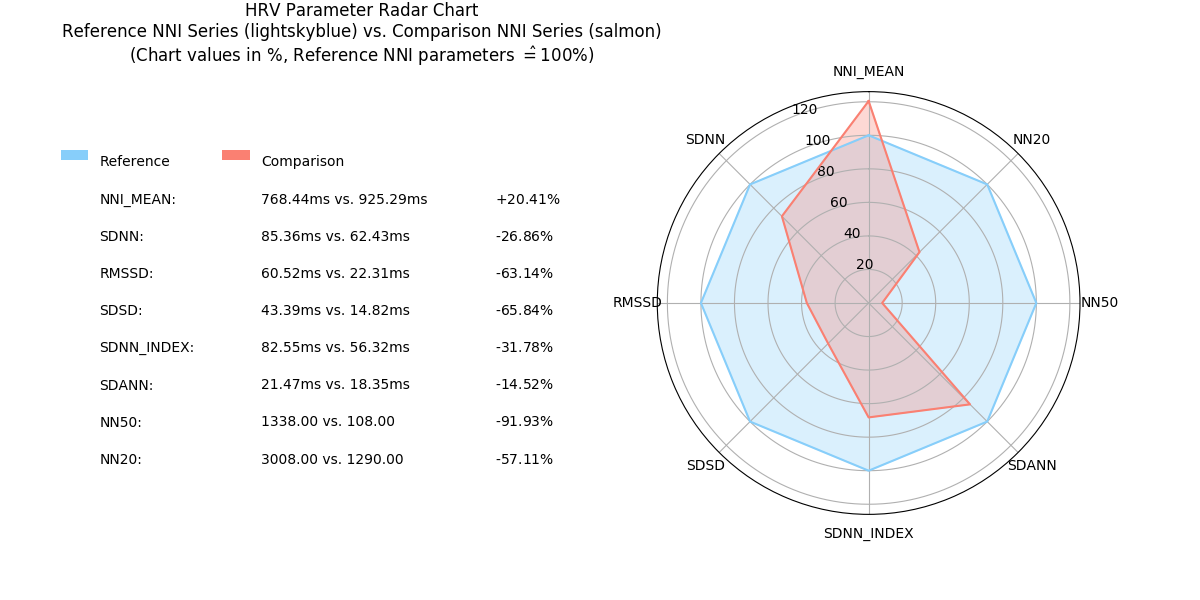
Sample Radar Chart plot with 8 parameters.

The radar_chart() function is not limited to a specific number of HRV parameters, as the Radar Chart will automatically be adjusted to the number of provided HRV parameters.

For instance, in the previous example, the input parameter list consisted of 8 HRV parameters. In the following example, the input parameter list consists of 5 parameters only:

# Specify the HRV parameters to be computed
     params = ['nni_mean', 'sdnn', 'rmssd', 'sdsd', 'nn50', 'nn20', 'sd1', 'fft_peak']

# Plot the Radar Chart
radar_chart(nni=ref_nni, comparison_nni=comparison_nni, parameters=params)

… which generates the following Radar Chart: